Big idea: If a terminal phase looks wrong visually, half-life is unreliable no matter what the number says.
Learning Objectives
By the end of this lesson, you will be able to:
Generate individual PK profile plots.
Use log-scale plots to evaluate terminal-phase behavior.
Visually identify poor lambda_z regions.
Detect suspicious profiles before performing NCA.
Key Ideas
Visual inspection is one of the most powerful QC tools in PK analysis.
Linear-scale plots help reveal overall exposure patterns .
Log-scale plots reveal the terminal log-linear region used to estimate \(\lambda_z\) .
Terminal slope diagnostics should always be confirmed visually .
Numerical outputs like half-life are only reliable if the terminal region is visually credible.
Setup: Prepare Example Data
library (tidyverse)data (Theoph)<- as_tibble (Theoph) %>% transmute (ID = Subject,TIME = Time,CONC = conc
# A tibble: 132 × 3
   ID     TIME  CONC
   <ord> <dbl> <dbl>
 1 1      0     0.74
 2 1      0.25  2.84
 3 1      0.57  6.57
 4 1      1.12 10.5
 5 1      2.02  9.66
 6 1      3.82  8.58
 7 1      5.1   8.36
 8 1      7.03  7.47
 9 1      9.05  6.89
10 1     12.1   5.94
# ℹ 122 more rows
Strategies
When reviewing PK profiles visually:
Start with a linear-scale plot to understand the full profile.
Then inspect a log-scale plot to evaluate the terminal decline.
Look specifically at the last several time points .
Confirm that the terminal phase appears approximately log-linear .
Flag profiles that look inconsistent or noisy.
Worked Example 1: Linear Profile Plot
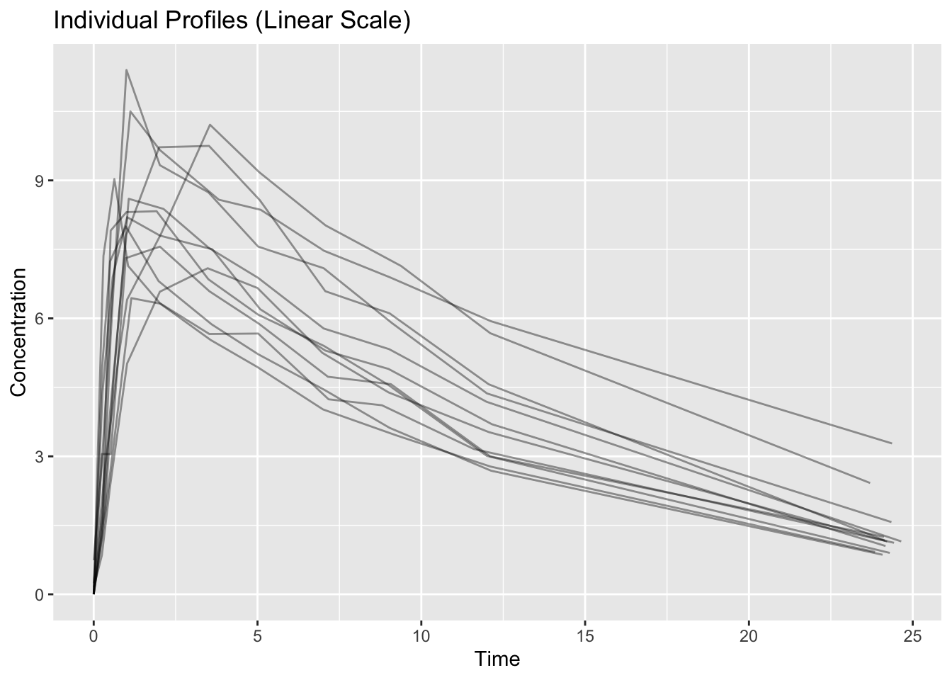
A linear-scale plot provides an overview of the full concentration-time profiles.
ggplot (conc_df, aes (TIME, CONC, group = ID)) + geom_line (alpha = 0.4 ) + labs (title = "Individual Profiles (Linear Scale)" ,x = "Time" ,y = "Concentration"
This plot helps reveal:
overall exposure patterns
potential outliers
unusual spikes or dips
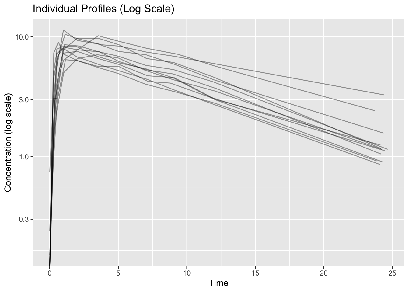
Worked Example 2: Log-Scale Profile Plot
Log-scale plots reveal the terminal phase used to estimate \(\lambda_z\) .
ggplot (conc_df, aes (TIME, CONC, group = ID)) + geom_line (alpha = 0.4 ) + scale_y_log10 () + labs (title = "Individual Profiles (Log Scale)" ,x = "Time" ,y = "Concentration (log scale)"
On a log scale, a well-behaved terminal phase should appear approximately linear .
What to Look For in Log Plots
A reliable terminal phase typically shows:
A clear log-linear decline
Several points forming a consistent slope
No upward curvature at the end
Minimal noise in the last samples
These visual signals support a stable \(\lambda_z\) estimate.
Common Mistakes
Trusting half-life estimates without visually checking the terminal region.
Ignoring noisy or upward-trending final samples.
Using too few points to define the terminal phase.
Overlooking time unit errors that distort the curve shape.
Practice Problems
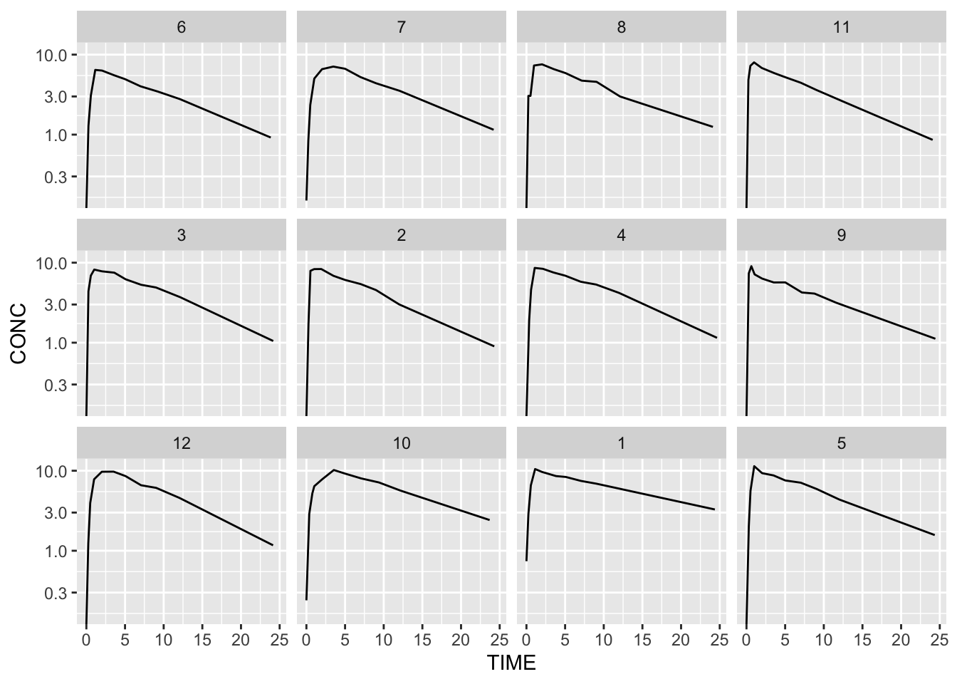
Executable: Create a faceted log-scale plot with one panel per subject.Executable: Identify subjects with unusually noisy terminal regions.Conceptual: Why does an upward final point distort \(\lambda_z\) estimation?
1. Faceted log-scale plot
ggplot (conc_df, aes (TIME, CONC)) + geom_line () + scale_y_log10 () + facet_wrap (~ ID)
2. Identifying noisy terminal regions
Visual inspection is typically used. Look for:
jagged terminal segments
upward final points
inconsistent slopes
3. Conceptual explanation
An upward final point violates the assumption of log-linear elimination. When included in the terminal regression, it flattens the slope, which inflates the half-life estimate.
Summary
Visual QC is a non-negotiable step before trusting terminal-phase metrics.
Reliable half-life estimation requires:
a clear log-linear terminal phase
adequate terminal sampling
visually consistent concentration decline
Numbers should confirm what the plot already suggests , not replace visual judgment.
Always inspect log-scale plots before trusting half-life.
Terminal phases should appear approximately linear on a log scale .
Watch closely for noisy final samples .
Visual QC should always precede automated NCA reporting.