Approaches to Population Analysis
Understand the major approaches used to analyze pharmacokinetic data across individuals, and why nonlinear mixed-effects modeling became the dominant framework.
Tip
What you’ll build today: a clear mental model of the main approaches to population analysis, what each one assumes, and why nonlinear mixed-effects modeling became the standard approach in pharmacometrics.
Learning Objectives
By the end of this lesson, you will be able to:
- Distinguish naive pooled, two-stage, and nonlinear mixed-effects approaches
- Explain why some approaches fail when variability matters
- Understand why sparse data changes the choice of method
- Connect modeling approach to the quality of scientific and dosing decisions
Key Ideas
Once you accept that patients differ, a new question appears:
How should those differences be analyzed?
That question led to several major approaches in pharmacometrics.
At a high level, these approaches differ in what they do with variability:
- ignore it
- estimate it after the fact
- model it directly
Insight: The history of population analysis is largely the history of learning that variability cannot be treated as an afterthought.
Warning
If the analysis approach does not represent variability appropriately, the model may fit the data and still support poor decisions.
Why This Lesson Matters
The same PK dataset can be analyzed in very different ways.
Those choices affect:
- parameter estimates
- uncertainty
- the ability to use sparse data
- how well decisions generalize to real patients
This is why “how you estimate” is not just technical detail.
It changes what the model can mean.
The Three Core Approaches
1. Naive Pooled Analysis
In naive pooled analysis, all observations are treated as if they came from a single individual.
That means:
- individual differences are ignored
- repeated measures from different people are pooled together
- one set of parameters is estimated from the combined data
What it assumes
It effectively assumes that:
- everyone behaves the same
- between-subject variability is negligible or irrelevant
Why it can be misleading
If variability is real, naive pooling can:
- blur true differences across individuals
- bias parameter estimates
- produce a smooth fit that represents nobody particularly well
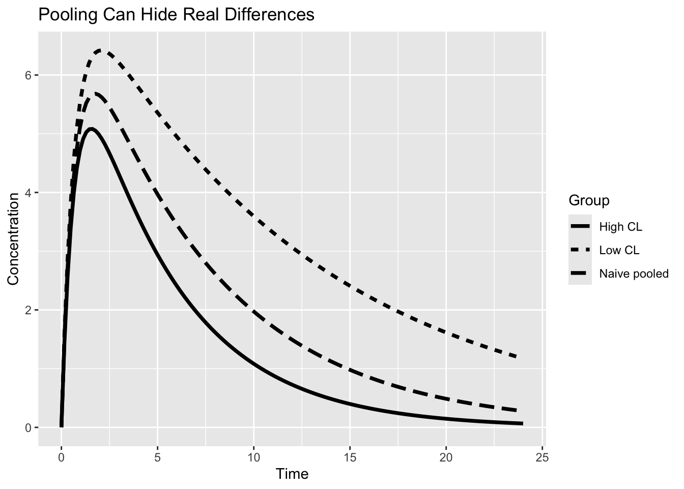
Worked Example: Why Naive Pooling Fails
Imagine two groups:
- low clearance patients
- high clearance patients
The pooled curve appears reasonable.
But it may not represent any real patient.
That becomes dangerous when decisions depend on extremes rather than averages.
2. Two-Stage Analysis
In a two-stage approach:
- Fit each subject individually
- Summarize the resulting parameters across subjects
This is conceptually appealing because it respects individuality.
What it does better than naive pooling
- preserves subject-specific estimates
- acknowledges that patients differ
What its limitations are
Two-stage methods can be unstable when:
- individual data are sparse
- some subjects have poorly estimated parameters
- those unstable individual estimates are then averaged
So although this approach is better than naive pooling conceptually, it may perform poorly in real studies with limited data.
Expanding the Example: Sparse Data Problem
Suppose each patient has only a few samples.
In a two-stage analysis:
- each subject is fit separately
- some subjects may have poorly estimated parameters
- those unstable estimates are then averaged
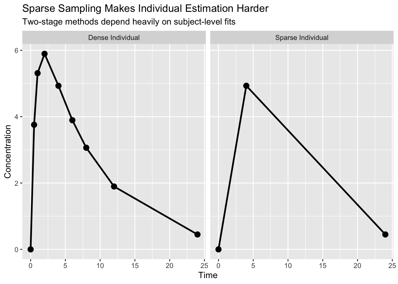
Compare the two situations.
With dense data:
- the individual profile is easier to estimate
With sparse data:
- many parameter combinations may explain the same observations
That uncertainty carries into the population summary.
This is one reason two-stage approaches often struggle in modern pharmacometrics.
The Real Question
Notice the progression:
Naive pooled asks:
“What profile best fits everyone?”
Two-stage asks:
“What are individual parameters?”
NLME asks:
“What population generated these observations?”
That shift changes pharmacometrics fundamentally.
3. Nonlinear Mixed-Effects (NLME) Modeling
NLME models estimate:
- typical population behavior
- variability across individuals
- residual unexplained error
all simultaneously.
A simple conceptual representation is:
\[ \theta_i = \theta_{typical} \cdot e^{\eta_i} \]
and observed data are then linked through a residual error model.
This framework allows the model to ask:
- What is typical?
- How much do individuals vary?
- How much uncertainty remains?
Visualizing How NLME Uses Sparse Data
Unlike two-stage methods, NLME does not estimate each subject independently.
Instead:
- subjects contribute information simultaneously
- stronger profiles help stabilize weaker profiles
- population information supports individual estimation
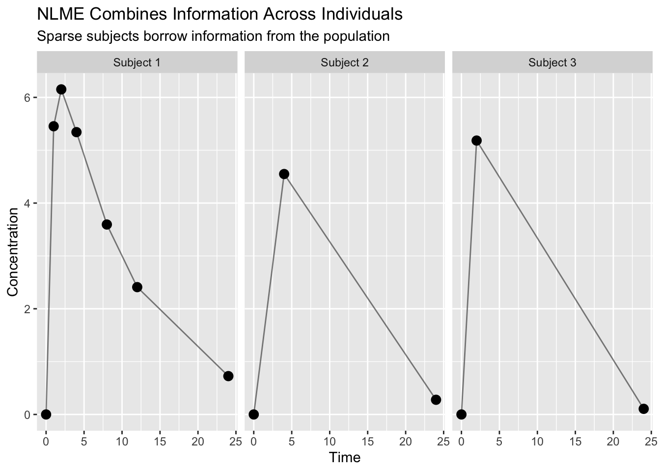
Notice:
- Subject 1 contributes rich information
- Subjects 2 and 3 are sparse
- NLME estimates all subjects together
This process is often called:
borrowing strength
because population information helps stabilize individual estimates.
Visualizing the Three Approaches
Each approach treats individual differences differently.
flowchart LR

A["Naive Pooled"]

-->

B["One Typical Fit"]

C["Two-Stage"]

-->

D["Fit Individuals"]

-->

E["Average Parameters"]

F["NLME"]

-->

G["Estimate Typical + Variability Together"]
Conceptually:
- Naive pooled → combine everyone first
- Two-stage → fit separately, summarize later
- NLME → estimate population and individuals simultaneously
Why NLME Became the Standard
NLME became dominant because it can:
- use sparse and dense data together
- separate typical values from variability
- borrow strength across subjects
- support realistic predictions for populations
This is especially important in pharmacometrics, where many studies do not provide rich data for every individual.
Insight: NLME is powerful because it estimates typical behavior and variability simultaneously.
Note
A useful question is: “Does this approach treat variability as part of the model—or as a nuisance after the model?”
A Simple Comparison
| Approach | Variability | Sparse Data | Decision Support |
|---|---|---|---|
| Naive pooled | Ignored | Poor | Weak |
| Two-stage | Estimated afterward | Limited | Moderate |
| NLME | Modeled directly | Strong | Strong |
The main difference is not complexity.
It is how variability is treated.
Decision Implications
These approaches do not just produce different parameter estimates.
They support different kinds of decisions.
Naive pooled
May suggest one “average” dose is fine.
Two-stage
May reveal subject differences, but estimate them unreliably.
NLME
Allows you to ask:
- what proportion of patients are likely above target?
- what proportion are likely below target?
- how much unexplained variability remains?
- should dose be individualized?
That is why NLME is not just statistically convenient.
It is decision-relevant.
Strategies
- Match the analysis approach to the data structure
- Be suspicious of methods that ignore variability
- Prefer approaches that can separate typical behavior from spread
- Ask what kind of decision the method can actually support
- Treat sparse data as a modeling challenge, not a reason to ignore individual differences
Common Mistakes
- Using naive pooled analysis when variability is substantial
- Assuming a good pooled fit represents real patients well
- Trusting two-stage summaries when individual fits are weak
- Thinking NLME is “more advanced” but not more meaningful
- Choosing an approach for convenience rather than for the scientific question
Practice Problems
- What does naive pooled analysis assume about variability?
- Why can two-stage analysis become unstable with sparse data?
- What does NLME estimate simultaneously?
- Why is NLME especially useful in pharmacometrics?
TipStep-by-Step Solutions
- It effectively assumes variability is negligible or can be ignored.
- Because weak individual fits can produce unstable subject-level parameters that distort the final summary.
- Typical population behavior, inter-individual variability, and residual unexplained error.
- Because it can use sparse data, represent variability directly, and support population-level decisions.
Summary
Population analysis approaches differ in how they treat variability.
- Naive pooled analysis ignores it
- Two-stage analysis estimates it indirectly
- NLME models it directly
That progression matters because pharmacometrics is fundamentally about understanding and managing differences across patients.
TipQuick Tips
- If variability matters, naive pooling is risky.
- Two-stage analysis can fail when individual data are weak.
- NLME models typical values and variability together.
- Sparse data often require stronger population methods, not simpler methods.
- Always ask what kind of decision the analysis approach can support.