Residuals and Goodness-of-Fit
Understand residuals, goodness-of-fit plots, and how they reveal problems in pharmacometric models.
Tip
What you’ll build today: the ability to interpret residuals and goodness-of-fit plots to diagnose model problems.
Learning Objectives
By the end of this lesson, you will be able to:
- Define residuals in pharmacometric models
- Interpret common goodness-of-fit plots
- Recognize patterns that indicate model misspecification
- Connect diagnostics to model assumptions
Key Ideas
After fitting a model, we compare:
- observed data
- model predictions
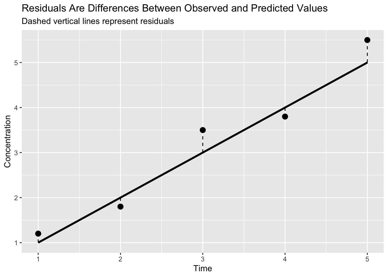
The difference is called a residual:
\[ \text{Residual} = \text{Observed} - \text{Predicted} \]
Residuals help answer:
How well does the model explain the data?
Types of Residuals
Raw Residuals
Raw residuals measure the direct difference between observation and prediction.
\[ RES = DV - PRED \]
Where:
- \(DV\) = observed value
- \(PRED\) = model prediction
Interpretation:
- positive residual → model underpredicts
- negative residual → model overpredicts
Weighted Residuals (WRES)
Weighted residuals scale residuals by expected variability.
Conceptually:
\[ WRES \approx \frac{DV-PRED} {SD} \]
Where:
- \(SD\) = standard deviation (the expected spread of observations)
This makes residuals:
- easier to compare across observations
- more interpretable when variability changes
Interpretation:
- values near zero → predictions align with expectations
- large positive or negative values → unusual prediction errors
Conditional Weighted Residuals (CWRES)
CWRES extend weighted residuals by accounting for:
- individual random effects (\(\eta\))
- population uncertainty
Conceptually:
\[ CWRES \approx \frac{DV-PRED} {\text{Conditional SD}} \]
Where:
- \(DV\) = observed value
- \(PRED\) = model prediction
- Conditional SD = the variability expected under the model for that specific observation
Unlike WRES, CWRES account for both:
- expected observation variability
- uncertainty introduced by individual and population effects
CWRES are commonly used in:
- population PK models
- residual diagnostics
- goodness-of-fit evaluation
Insight: CWRES ask whether observations are unusual given the model and expected variability.
Worked Example: Residual Concept
A residual is the vertical difference between an observed value and the model prediction.
Each residual measures:
\[ \text{Residual} = \text{Observed} - \text{Predicted} \]
Positive residuals mean observations are above predictions.
Negative residuals mean observations are below predictions.
Goodness-of-Fit (GOF) Plots
Common plots include:
Observed vs Predicted
- Should lie along identity line
Residuals vs Time
- Should show no pattern
Residuals vs Predictions
- Should be randomly scattered
Expanding the Idea: What Patterns Mean
Residual plots are useful because different patterns suggest different problems.
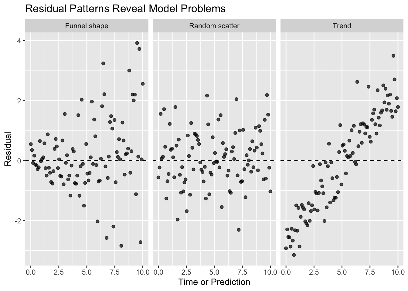
Interpretation:
- Random scatter → residual behavior looks acceptable
- Trend → model may be missing time-dependent structure
- Funnel shape → residual variability changes with magnitude
The goal is not to make residuals zero.
The goal is to remove systematic structure.
Insight
Residuals should look like random noise—patterns indicate problems.
Note
A useful model does not produce perfect residuals.
It produces residuals with no meaningful systematic structure.
Why This Matters
Residual diagnostics help detect:
- model misspecification
- incorrect variability assumptions
- poor predictive performance
Strategies
- Always inspect multiple GOF plots
- Look for patterns, not individual points
- Combine visual and statistical checks
Common Mistakes
- Ignoring residual patterns
- Overreacting to single outliers
- Assuming fit is good without diagnostics
Practice Problems
- What is a residual?
- What should residual plots look like?
- What does a trend indicate?
TipStep-by-Step Solutions
- Observed minus predicted
- Random scatter with no pattern
- Model misspecification
Summary
Residuals:
- measure model fit
- reveal patterns
- diagnose problems
TipQuick Tips
- Residuals should look random
- Patterns = problems
- Use multiple plots
- Focus on trends, not noise