flowchart TB

TV["Typical Value (θtypical)"]
COV["Covariates"]
IND["Individual Parameter (θi)"]
PRED["Prediction"]
OBS["Observed Data"]

ETA["Random Effect (η)"]
EPS["Residual Error (ε)"]

TV --> IND
COV --> IND
ETA -. modifies .-> IND
IND --> PRED
PRED --> OBS
EPS -. perturbs .-> OBS
Covariates, Random Effects, and Hierarchical Modeling
Understand how covariates, random effects, and residual error models work together in hierarchical population models.
Tip
What you’ll build today: a complete mental model of how individual parameters and observations are formed from typical values, covariates, random effects, and residual error.
Learning Objectives
By the end of this lesson, you will be able to:
- distinguish fixed effects, covariate effects, random effects, and residual error
- explain how individual parameters are constructed in hierarchical models
- compare common inter-individual variability models
- compare common residual error models
- interpret continuous and categorical covariate model structures
- connect covariates, variability, exposure, and decisions
Key Ideas
Population models combine:
- typical values
- covariate effects
- random effects
- residual error
A common individual-parameter structure is:
\[ \theta_i = \theta_{typical} \cdot f(COV_i) \cdot \exp(\eta_i) \]
Interpretation:
Individual behavior = typical behavior + explained variability + unexplained variability
Warning
If you ignore covariates, systematic variability may appear random.
Visualizing Hierarchical Modeling
Interpretation:
- \(\theta_{typical}\) → expected population value
- covariates → systematic differences
- \(\eta\) → remaining individual variability
- \(\epsilon\) → observation-level variability
Building Individual Parameters
Individual parameters are built in stages:
Typical Value → Covariate Adjustment → Random Effect → Individual ParameterConceptually:
\[ \theta_i = \theta_{typical} \times Covariate\ Effect \times \exp(\eta_i) \]
This structure is central to hierarchical or mixed-effects modeling.
Fixed Effects, Covariates, Random Effects, and Residual Error
| Component | Meaning |
|---|---|
| Fixed effect | typical population value |
| Covariate effect | systematic difference explained by measured information |
| Random effect | unexplained subject-level difference |
| Residual error | observation-level disagreement |
These components answer different questions.
Typical value → What is usual?
Covariate effect → What systematic difference can we explain?
Random effect → What subject-level difference remains?
Residual error → What observation-level disagreement remains?
Random Effects (\(\eta\))
Random effects describe variability not explained by measured covariates.
A common structure is:
\[ \theta_i = \theta_{typical} \exp(\eta_i) \]
where:
\[ \eta_i \sim N(0,\omega^2) \]
Interpretation:
- \(\eta_i > 0\) → larger-than-typical parameter
- \(\eta_i < 0\) → smaller-than-typical parameter
- \(\omega^2\) → magnitude of inter-individual variability
Exponential random effects are common because they preserve positive parameters.
Inter-Individual Variability Models
Inter-individual variability can be modeled using different structures.
Assume clearance depends on a continuous covariate such as creatinine clearance, \(CrCl_i\).
Additive IIV Model
(constant variance)
\[ CL_i = \theta_1 + \theta_2 CrCl_i + \eta_i \]
Interpretation:
- \(\eta_i\) adds a fixed amount
- variability is on the original parameter scale
- variability does not scale with the magnitude of clearance
This can be simple but may allow impossible values such as negative clearance.
Proportional IIV Model
(constant coefficient of variation)
\[ CL_i = (\theta_1 + \theta_2 CrCl_i)(1+\eta_i) \]
Interpretation:
- variability scales with the typical value
- larger clearance values have larger absolute variability
This is more realistic than additive variability for many positive PK parameters.
Exponential IIV Model
(constant CV, log-normal variability)
\[ CL_i = (\theta_1 + \theta_2 CrCl_i)\exp(\eta_i) \]
Equivalent log form:
\[ \log(CL_i)= \log(\theta_1 + \theta_2 CrCl_i)+ \eta_i \]
Interpretation:
- preserves positivity
- implies log-normal variability
- common in population PK modeling
This is one of the most common IIV forms for clearance and volume.
Residual Variability Models
Residual variability describes differences between predictions and observed data.
Let:
- \(Y_{ij}\) = observation for subject \(i\) at time \(j\)
- \(F_{ij}\) = model prediction for subject \(i\) at time \(j\)
- \(\epsilon_{ij}\) = residual error
Additive Residual Error
(homoscedastic, constant variance)
\[ Y_{ij}=F_{ij}+\epsilon_{ij} \]
Interpretation:
- same absolute error across the prediction range
- useful when measurement noise is roughly constant
Example:
Prediction = 2 → error about ±0.5
Prediction = 20 → error about ±0.5
Proportional Residual Error
(heteroscedastic, constant CV)
\[ Y_{ij}=F_{ij}(1+\epsilon_{ij}) \]
Interpretation:
- error increases with prediction magnitude
- useful when variability is relative or percentage-based
Example:
Prediction = 2 → 10% error is ±0.2
Prediction = 20 → 10% error is ±2
Exponential Residual Error
(approximately constant CV)
\[ Y_{ij}=F_{ij}\exp(\epsilon_{ij}) \]
Equivalent log form:
\[ \log(Y_{ij})=\log(F_{ij})+\epsilon_{ij} \]
Interpretation:
- residual error is additive on the log scale
- preserves positive observations
- common for concentration data
Combined Additive and Proportional Error
\[ Y_{ij}=F_{ij}(1+\epsilon_{1ij})+\epsilon_{2ij} \]
Interpretation:
- proportional error dominates at larger values
- additive error can help at lower values
- flexible for concentration-time data
Covariates Explain Systematic Variability
Covariates explain systematic differences between individuals.
Before covariates:
Total variability = unexplained variabilityAfter covariates:
Total variability = explained variability + unexplained variabilityCovariates reduce unexplained variability, but they rarely eliminate it.
Continuous Covariate Models
Continuous covariates include:
WT, AGE, CLCR, ALBA common target parameter is clearance.
Linear Additive
\[ TVCL=\theta_1+\theta_2WT_i \]
\[ CL_i=TVCL\exp(\eta_i) \]
Interpretation:
- \(\theta_1\) → intercept
- \(\theta_2\) → fixed change per unit of weight
This model is simple but can be sensitive to units.
Linear Centered
\[ TVCL=\theta_1+\theta_2(WT_i-WT_{ref}) \]
\[ CL_i=TVCL\exp(\eta_i) \]
Interpretation:
- \(\theta_1\) → typical clearance at \(WT_{ref}\)
- \(\theta_2\) → change in clearance per unit above or below \(WT_{ref}\)
Centering improves interpretability.
Power Model
\[ TVCL=\theta_1WT_i^{\theta_2} \]
\[ CL_i=TVCL\exp(\eta_i) \]
Interpretation:
- \(\theta_2\) controls nonlinear scaling
- relative changes are emphasized
Normalized Power Model
\[ TVCL= \theta_1 \left( \frac{WT_i}{WT_{ref}} \right)^{\theta_2} \]
\[ CL_i=TVCL\exp(\eta_i) \]
Interpretation:
- \(WT=WT_{ref}\) → no adjustment
- \(WT>WT_{ref}\) → effect depends on \(\theta_2\)
- \(WT<WT_{ref}\) → effect depends on \(\theta_2\)
This is one of the most common continuous covariate structures in PK.
Log-Transformed Power Model
\[ LNCL= \theta_1+ \theta_2 \log\left(\frac{WT_i}{WT_{ref}}\right)+ \eta_i \]
\[ CL_i=\exp(LNCL) \]
Interpretation:
This is the normalized power model written on the log scale.
It is often convenient when parameters are modeled using log transformations.
Categorical Covariate Models
Categorical covariates include:
SEX, FORMULATION, DISEASE GROUPAssume:
- \(SEX_i=0\) → Female
- \(SEX_i=1\) → Male
Linear Additive
\[ TVCL=\theta_1+\theta_2SEX_i \]
\[ CL_i=TVCL\exp(\eta_i) \]
Interpretation:
- \(\theta_2\) is an absolute group difference
Linear Proportional
\[ TVCL=\theta_1(1+\theta_2SEX_i) \]
\[ CL_i=TVCL\exp(\eta_i) \]
Interpretation:
- \(\theta_2\) is a relative group difference
- \(\theta_2=0.2\) → 20% higher \(TVCL\) when \(SEX=1\)
Power Model
\[ TVCL=\theta_1\theta_2^{SEX_i} \]
\[ CL_i=TVCL\exp(\eta_i) \]
Interpretation:
- \(SEX=0\) → \(TVCL=\theta_1\)
- \(SEX=1\) → \(TVCL=\theta_1\theta_2\)
This represents a multiplicative group effect.
Log-Transformed Power Model
\[ LNCL=\theta_1+SEX_i\log(\theta_2)+\eta_i \]
\[ CL_i=\exp(LNCL) \]
Interpretation:
This is the categorical power model written on the log scale.
Worked Example: Weight Explains Part of Variability
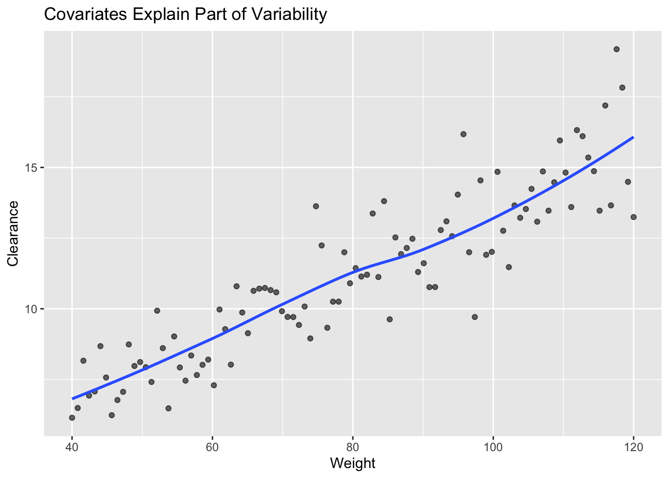
Interpretation:
- heavier subjects tend to have larger clearance
- individuals still vary around the trend
- weight explains part of variability
- \(\eta\) explains what remains
Residual Error Is Different From Random Effects
Random effects act on individual parameters.
Residual error acts on observations.
Random effects → subject-level variability
Residual error → observation-level variability
Both are needed.
Full Hierarchical Model
A population model can be viewed as:
Population value → Covariates → Random effects → Prediction → Residual error → ObservationThis structure allows us to:
- explain variability
- predict individual behavior
- quantify uncertainty
- support decisions
Insight
Covariates improve explanation and prediction.
Random effects and residual error quantify what remains unexplained.
Note
Always ask: What variability can I explain, and what variability remains?
Strategies
- use biologically plausible covariates
- prefer simple, interpretable forms
- distinguish IIV from residual error
- evaluate whether variability is actually reduced
Common Mistakes
- adding covariates without justification
- overinterpreting weak relationships
- ignoring unexplained variability
- confusing random effects with residual error
Practice Problems
What are the four major components of a hierarchical population model?
Why are exponential random effects commonly used for PK parameters?
Compare additive, proportional, and exponential IIV models.
Compare additive, proportional, and combined residual error models.
Why do covariates usually not eliminate \(\eta\)?
TipStep-by-Step Solutions
Problem 1
The major components are:
- typical values
- covariate effects
- random effects
- residual error
Problem 2
Exponential random effects preserve positivity and produce log-normal variability.
This is useful for parameters such as clearance and volume.
Problem 3
Additive IIV adds a fixed amount.
Proportional IIV scales with the typical value.
Exponential IIV scales multiplicatively and preserves positivity.
Problem 4
Additive residual error assumes constant absolute error.
Proportional residual error assumes constant relative error.
Combined error allows both behaviors.
Problem 5
Covariates explain measured systematic differences.
Unmeasured differences and biological variability usually remain.
Summary
Hierarchical models combine:
- typical behavior
- covariate effects
- inter-individual variability
- residual variability
Together these support:
- interpretation
- prediction
- uncertainty quantification
- decision-making
TipQuick Tips
- Covariates explain systematic variability
- \(\eta\) captures remaining subject variability
- \(\epsilon\) captures observation variability
- IIV and residual error are different
- Always separate explanation from uncertainty