Population Thinking in Pharmacometrics
Understand how population models describe both typical behavior and variability, and how this drives decision-making.
Tip
What you’ll build today: the ability to think in terms of populations and distributions rather than single “typical” values.
Learning Objectives
By the end of this lesson, you will be able to:
- Define population modeling in pharmacometrics
- Distinguish typical vs individual parameter values
- Interpret random effects (η) conceptually
- Connect population thinking to real decisions
Key Ideas
Population models describe two things simultaneously:
- Typical behavior (what is expected on average)
- Variability (how individuals differ from that average)
A common representation:
\[ \theta_i = \theta_{typical} \cdot e^{\eta_i} \]
Conceptually:
- \(\theta_{typical}\) sets the center
- \(\eta_i\) determines where an individual sits relative to that center
In pharmacometrics, \(\eta_i\) is often called an:
individual random effect
Insight: Every individual has their own parameter value — there is no single “true” value for all patients.
Warning
The typical value is not “the value” — it is just the center of a distribution.
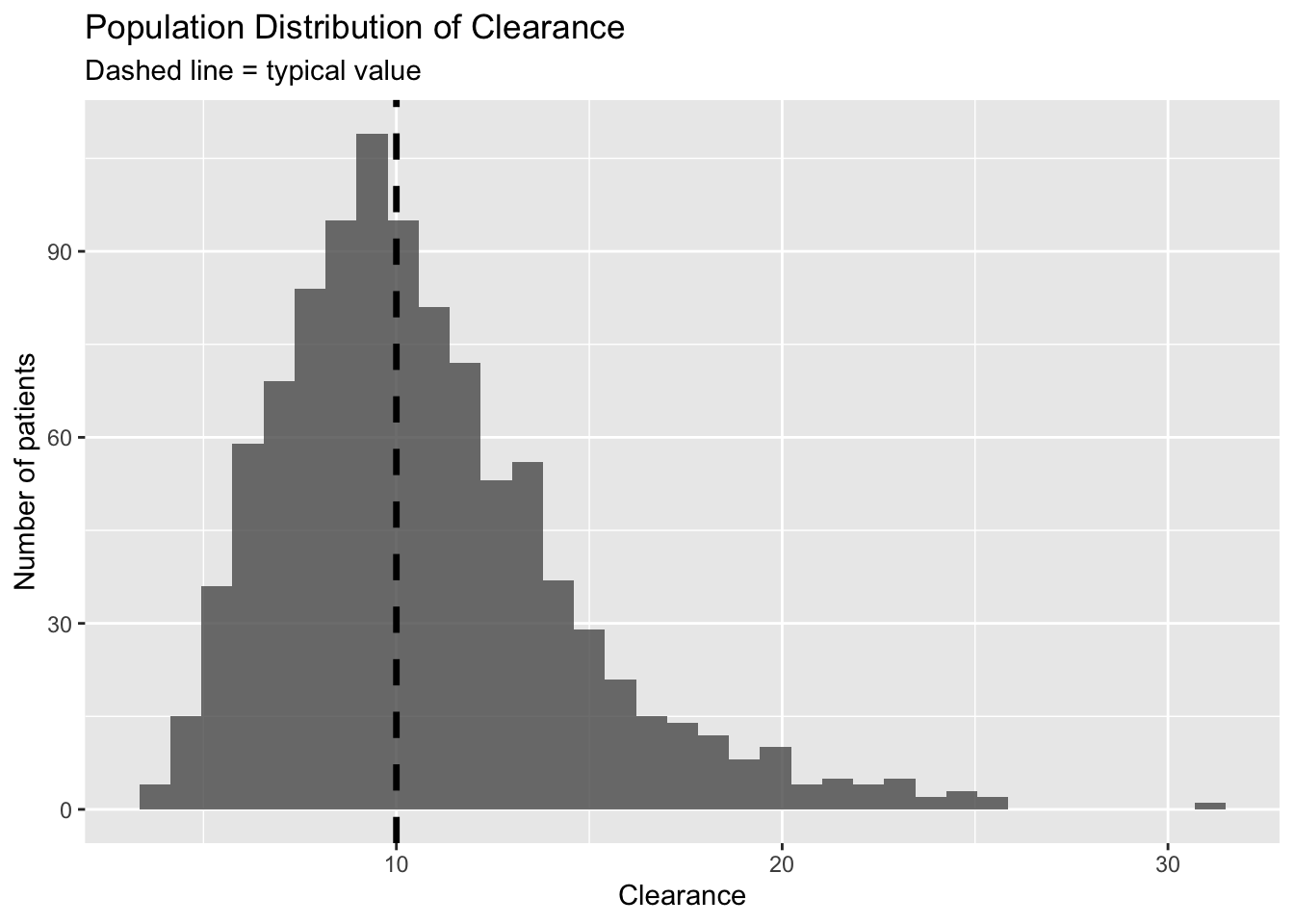
Worked Example: Distribution of Clearance
Suppose the typical clearance is:
\[ CL_{typical}=10 \]
But individuals vary around that value.
Notice:
- many patients are near the typical value
- some are much lower
- some are much higher
Now connect this to exposure:
- lower CL → higher AUC
- higher CL → lower AUC
Same dose.
Different outcomes.
Expanding the Example: From Values to Distributions
Population thinking changes the questions we ask.
Instead of:
“What is clearance?”
we ask:
“Where does this patient fall in the population?”
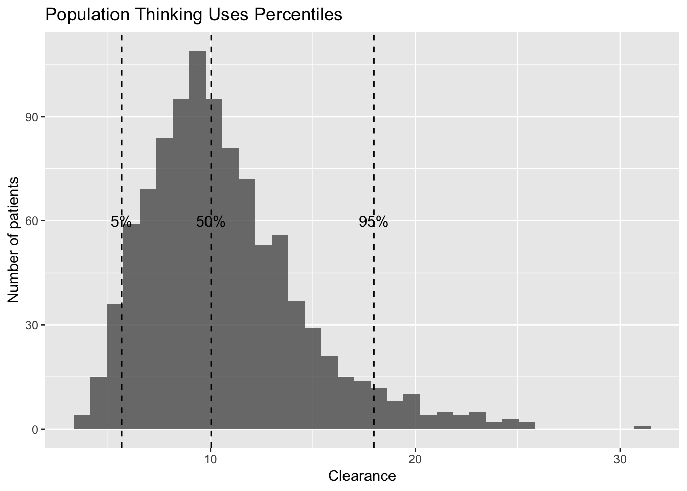
This allows questions such as:
- What is the 5th percentile?
- What is the median?
- What fraction exceeds a threshold?
That is the foundation of population decision-making.
Insight
Population thinking changes the question from:
“What is the value?”
to:
“What is the distribution of values?”
Note
Clinical decisions depend on probabilities, not single numbers.
Visualizing Population Thinking
Population models describe populations as distributions rather than single values.
flowchart TB

TV["Typical Value<br>(θtypical)"]

-->

DIST["Population Distribution"]

-->

IND["Individual Patients"]
Interpretation:
- θtypical defines the center
- variability creates a distribution
- each patient occupies a different position
Population models describe both:
- what is typical
- how individuals vary
Covariates (next lesson) help explain why patients occupy different positions.
Why This Matters for Decisions
Population models allow you to:
- estimate the probability of toxicity
- estimate the probability of efficacy
- evaluate whether a dose is appropriate for most patients
Example:
- Narrow distribution → predictable outcomes
- Wide distribution → high uncertainty and risk
Strategies
- Always interpret both center and spread
- Think in terms of percentiles and probabilities
- Connect variability to clinical outcomes
- Avoid relying on single values
Common Mistakes
- Treating the typical value as universal
- Ignoring distribution width
- Making decisions based on averages only
- Underestimating variability impact
Practice Problems
- What does \(\theta_{typical}\) represent?
- What does \(\eta_i\) represent?
- Why is population thinking important for dosing decisions?
TipStep-by-Step Solutions
- The central tendency of the parameter in the population
- The deviation of an individual from the typical value
- Because dosing decisions depend on how many patients fall outside target exposure
Summary
Population models describe:
- what is typical
- how much individuals vary
Together, these determine:
- exposure distributions
- response variability
- decision outcomes
Population models convert variability into probabilities and decisions.
TipQuick Tips
- Typical ≠ universal
- Always think in distributions
- Variability determines risk
- Decisions are probabilistic
- Focus on spread, not just center