library(tidyverse)Pipes and Readable Code
Learn how to write readable, PMx-friendly R code using pipes: build clear data workflows step-by-step.
Tip
Big idea: Pipes help you write code the way you think about workflows:
start with data → apply a sequence of clear steps → get a result you can trust.
Learning Objectives
By the end of this lesson, you will be able to:
- Explain what a pipe does conceptually.
- Read a pipe chain from top to bottom.
- Write clean pipelines using
%>%and tidyverse verbs. - Decide when to break a pipeline into intermediate objects.
- Avoid common “pipe abuse” patterns.
Setup
What a Pipe Does
A pipe takes the output of the left-hand side and passes it as the first argument to the next function.
Conceptually:
data %>% f()is similar to:
f(data)This matters because PMx workflows are typically a series of steps.
A PMx-Style Dataset
pk <- tibble(
  ID   = c(1, 1, 1, 2, 2, 2, 3, 3, 3),
  TIME = c(0.5, 1, 2, 0.5, 1, 2, 0.5, 1, 2),
  DV   = c(2.1, 3.8, 3.0, 1.6, 2.9, 2.4, 4.8, 7.2, 6.9)
)

pk
# A tibble: 9 × 3
ID TIME DV
<dbl> <dbl> <dbl>
1 1 0.5 2.1
2 1 1 3.8
3 1 2 3
4 2 0.5 1.6
5 2 1 2.9
6 2 2 2.4
7 3 0.5 4.8
8 3 1 7.2
9 3 2 6.9Reading Pipelines (A Key Skill)
Try reading this aloud:
pk %>%
  filter(TIME <= 1) %>%
  group_by(ID) %>%
  summarise(mean_DV = mean(DV), .groups = "drop")
# A tibble: 3 × 2
ID mean_DV
<dbl> <dbl>
1 1 2.95
2 2 2.25
3 3 6 “Start with pk, keep time ≤ 1, group by ID, compute mean DV.”
That’s what we want.
Pipes vs Nested Functions
Nested functions can get hard to read:
summarise(
  group_by(
    filter(pk, TIME <= 1),
    ID
  ),
  mean_DV = mean(DV)
)
# A tibble: 3 × 2
ID mean_DV
<dbl> <dbl>
1 1 2.95
2 2 2.25
3 3 6 Pipes are usually clearer.
One Step per Line (PMx readability standard)
Good:
pk %>%
  filter(TIME <= 1) %>%
  group_by(ID) %>%
  summarise(mean_DV = mean(DV), .groups = "drop")
# A tibble: 3 × 2
ID mean_DV
<dbl> <dbl>
1 1 2.95
2 2 2.25
3 3 6 Avoid cramming too much into one line.
When to Create an Intermediate Object
Intermediate objects improve debugging and QC.
pk_early <- pk %>% filter(TIME <= 1)

pk_summary <- pk_early %>%
  group_by(ID) %>%
  summarise(mean_DV = mean(DV), .groups = "drop")

pk_summary
# A tibble: 3 × 2
ID mean_DV
<dbl> <dbl>
1 1 2.95
2 2 2.25
3 3 6
Note
If you want to inspect intermediate outputs, save them.
A PMx Workflow Example: Quick QC Summary
Compute:
- number of observations per subject
- max concentration per subject
pk %>%
  group_by(ID) %>%
  summarise(
    n_obs = n(),
    max_DV = max(DV),
    .groups = "drop"
  )
# A tibble: 3 × 3
ID n_obs max_DV
<dbl> <int> <dbl>
1 1 3 3.8
2 2 3 2.9
3 3 3 7.2Pipes and Plotting
Pipes work nicely with ggplot too (we’ll cover ggplot in depth later — here we just show how pipes pass data into a plot):
pk %>%
  filter(ID %in% c(1, 2)) %>%
  ggplot(aes(TIME, DV, group = ID)) +
  geom_line() +
  geom_point() +
  theme_minimal()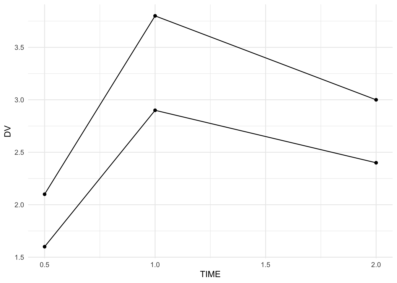
Strategies
- Use one operation per line.
- Save intermediate objects when you need QC checkpoints.
- Name objects based on what they represent (
pk_clean,pk_summary). - Keep pipelines short and focused.
- Prefer clarity over cleverness.
Practice Problems
- Filter
pktoTIME <= 1. - Compute mean DV by subject for
TIME <= 1. - Create
pk_earlyas an intermediate object and repeat the summary. - Create a plot for IDs 1 and 2 only.
- Rewrite a nested function version into a pipeline.
TipStep-by-Step Solutions
pk %>%
  filter(TIME <= 1)
# A tibble: 6 × 3
ID TIME DV
<dbl> <dbl> <dbl>
1 1 0.5 2.1
2 1 1 3.8
3 2 0.5 1.6
4 2 1 2.9
5 3 0.5 4.8
6 3 1 7.2pk %>%
filter(TIME <= 1) %>%
group_by(ID) %>%
summarise(mean_DV = mean(DV), .groups = "drop")# A tibble: 3 × 2
ID mean_DV
<dbl> <dbl>
1 1 2.95
2 2 2.25
3 3 6 pk_early <- pk %>% filter(TIME <= 1)
pk_early %>%
group_by(ID) %>%
summarise(mean_DV = mean(DV), .groups = "drop")# A tibble: 3 × 2
ID mean_DV
<dbl> <dbl>
1 1 2.95
2 2 2.25
3 3 6 pk %>%
filter(ID %in% c(1, 2)) %>%
ggplot(aes(TIME, DV, group = ID)) +
geom_line() +
geom_point() +
theme_minimal()
Summary
You now know how to:
- read and write pipelines clearly
- structure multi-step PMx data workflows
- choose when to save intermediate objects
- keep code review-friendly and reproducible
Pipes aren’t magic — they’re a readability tool. Use them with discipline.
TipQuick Tips
- Read pipelines like sentences.
- One transformation per line.
- Save checkpoints when debugging.
- If it’s hard to read, refactor.