library(tidyverse)
library(nlme)

data(Theoph)

terminal_data <- Theoph %>%
  filter(Time >= 4) %>%
mutate(log_conc = log(conc))Mixed-Effects Models in Practice with lme()
From Pooled Regression to Hierarchical PK Modeling (Theoph Terminal Phase)
Learning Objectives
By the end of this lesson, you will be able to:
- Fit and interpret linear mixed-effects models using
lme() - Distinguish fixed effects from random effects in PK terms
- Explain the difference between conditional (
fitted()) and marginal (predict(level=0)) predictions - Visually compare pooled and hierarchical fits
- Perform and interpret core diagnostics for mixed-effects models
- Translate model output into biological interpretation (elimination variability)
Key Ideas
- PK concentration–time data are hierarchical by design.
- Fixed effects represent the population-average trajectory.
- Random effects represent systematic subject-level deviations.
- Mixed-effects models model correlation induced by repeated measures.
- Diagnostics are required to validate structural and distributional assumptions.
Worked Example 1: Prepare Terminal Phase Data
We focus on the log-linear terminal phase of Theoph.
Visualize:
ggplot(terminal_data, aes(Time, log_conc, group = Subject)) +
  geom_point() +
  geom_line(alpha = 0.6) +
  labs(title = "Terminal Phase (Log Scale) by Subject")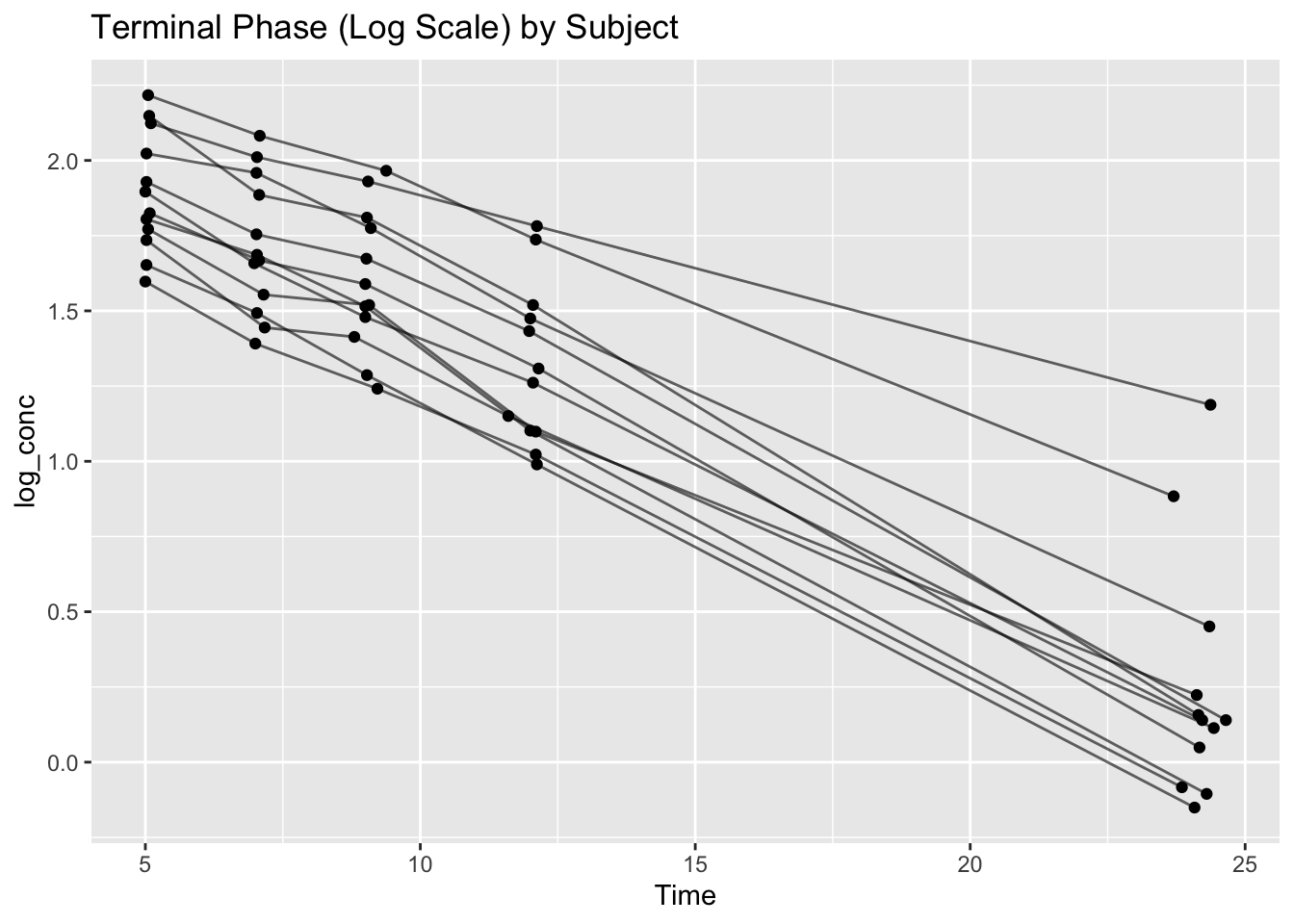
Observe:
- Roughly linear decline per subject
- Clear slope differences
- Clear intercept differences
This motivates hierarchical modeling.
Worked Example 2: Pooled Linear Model
lm_pooled <- lm(log_conc ~ Time, data = terminal_data)
summary(lm_pooled)
Call:
lm(formula = log_conc ~ Time, data = terminal_data)

Residuals:
    Min      1Q  Median      3Q     Max
-0.4230 -0.1975 -0.0535  0.2047  0.9406

Coefficients:
             Estimate Std. Error t value Pr(>|t|)
(Intercept)  2.343802   0.069087   33.92   <2e-16 ***
Time        -0.086031   0.005185  -16.59   <2e-16 ***
---
Signif. codes:  0 '***' 0.001 '**' 0.01 '*' 0.05 '.' 0.1 ' ' 1

Residual standard error: 0.2719 on 58 degrees of freedom
Multiple R-squared:  0.826, Adjusted R-squared:  0.823
F-statistic: 275.3 on 1 and 58 DF, p-value: < 2.2e-16terminal_data$fitted_lm <- fitted(lm_pooled)This assumes:
- One common elimination slope
- Independent residuals
- No subject-level variability
Biologically unrealistic.
Worked Example 3: Random Intercept Model
lme_intercept <- lme(
  log_conc ~ Time,
  random = ~ 1 | Subject,
  data = terminal_data
)

summary(lme_intercept)
Linear mixed-effects model fit by REML
Data: terminal_data
AIC BIC logLik
-27.3941 -19.15233 17.69705
Random effects:
Formula: ~1 | Subject
(Intercept) Residual
StdDev: 0.2508497 0.119405
Fixed effects: log_conc ~ Time
Value Std.Error DF t-value p-value
(Intercept) 2.3449775 0.07851322 47 29.86730 0
Time -0.0861333 0.00227713 47 -37.82536 0
Correlation:
(Intr)
Time -0.333
Standardized Within-Group Residuals:
Min Q1 Med Q3 Max
-2.08395490 -0.46560444 0.03446807 0.38916641 4.24096360
Number of Observations: 60
Number of Groups: 12 Here:
~ 1means each subject gets their own intercept| Subjectmeans those intercept deviations are grouped by subject
So the model allows each subject to start at a different baseline level, while still sharing one common population slope.
Worked Example 4: Random Intercept + Random Slope Model
lme_slope <- lme(
  log_conc ~ Time,
  random = ~ Time | Subject,
  data = terminal_data
)

summary(lme_slope)
Linear mixed-effects model fit by REML
Data: terminal_data
AIC BIC logLik
-71.93471 -59.57205 41.96736
Random effects:
Formula: ~Time | Subject
Structure: General positive-definite, Log-Cholesky parametrization
StdDev Corr
(Intercept) 0.19602203 (Intr)
Time 0.01451625 -0.017
Residual 0.05390312
Fixed effects: log_conc ~ Time
Value Std.Error DF t-value p-value
(Intercept) 2.3445510 0.05822154 47 40.26948 0
Time -0.0861095 0.00431482 47 -19.95669 0
Correlation:
(Intr)
Time -0.065
Standardized Within-Group Residuals:
Min Q1 Med Q3 Max
-1.6271612 -0.5798011 -0.0683255 0.5267383 1.6476914
Number of Observations: 60
Number of Groups: 12 Here:
Timemeans the model allows subject-specific slopes- The intercept is included automatically
| Subjectgroups those deviations by subject
So each subject can have:
- Their own baseline concentration
- Their own elimination slope
Interpretation:
- Fixed slope → population-average elimination rate
- Random slope variance → between-subject variability in elimination (
ke) - Random intercept variance → baseline variability
Conditional vs Marginal Predictions
Add predictions:
terminal_data <- terminal_data %>%
  mutate(
    fitted_lme_subject = fitted(lme_slope),
    fitted_lme_population = predict(lme_slope, level = 0)
)fitted()→ includes subject random effects (conditional)predict(level=0)→ population-average (marginal)
Population vs Individual Predictions
ggplot(terminal_data, aes(Time, log_conc)) +
  geom_point() +
  geom_line(aes(y = fitted_lme_subject)) +
  geom_line(aes(y = fitted_lme_population), linetype = 2) +
  facet_wrap(~ Subject) +
  labs(title = "Individual (solid) vs Population (dashed)")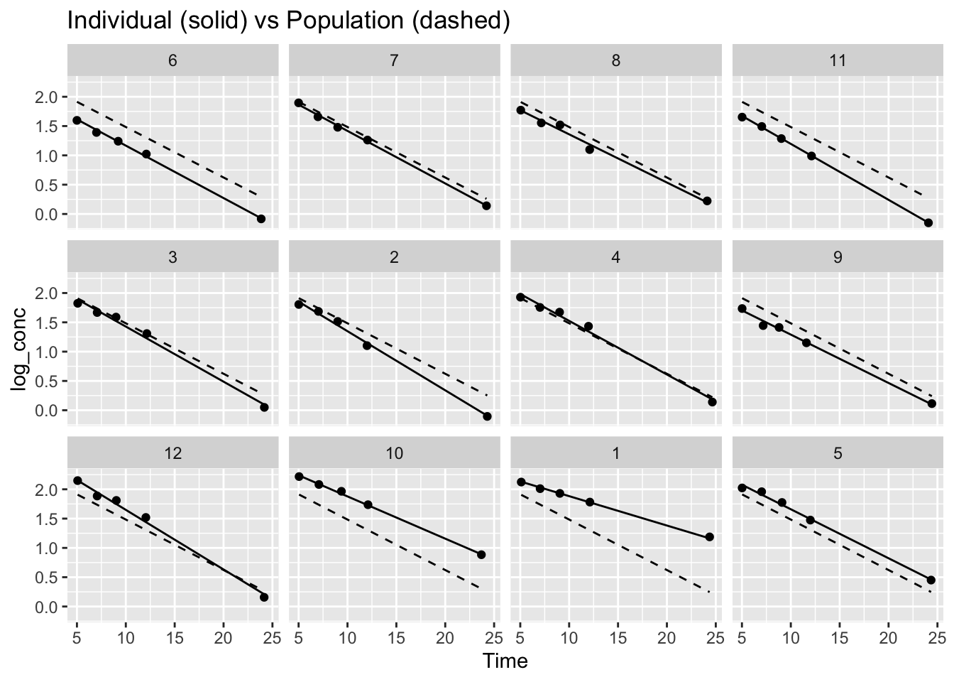
In each panel:
- Solid lines are subject-specific predictions
- Dashed lines are population-average predictions
Notice:
- The population line is the same structural trend for everyone
- Subject-specific lines adapt to each individual’s data
- Subjects with limited information are pulled closer to the population trend
This is the core idea of borrowing strength:
Individual estimates are informed by both the subject’s own data and the overall population structure.
This also leads to shrinkage, where extreme individual estimates are partially pulled toward the population average when information is limited.
Diagnostics
Residuals vs Fitted
terminal_data %>%
  mutate(resid = resid(lme_slope, type = "pearson")) %>%
  ggplot(aes(fitted_lme_subject, resid)) +
  geom_point() +
  geom_hline(yintercept = 0, linetype = 2) +
  labs(title = "Residuals vs Fitted")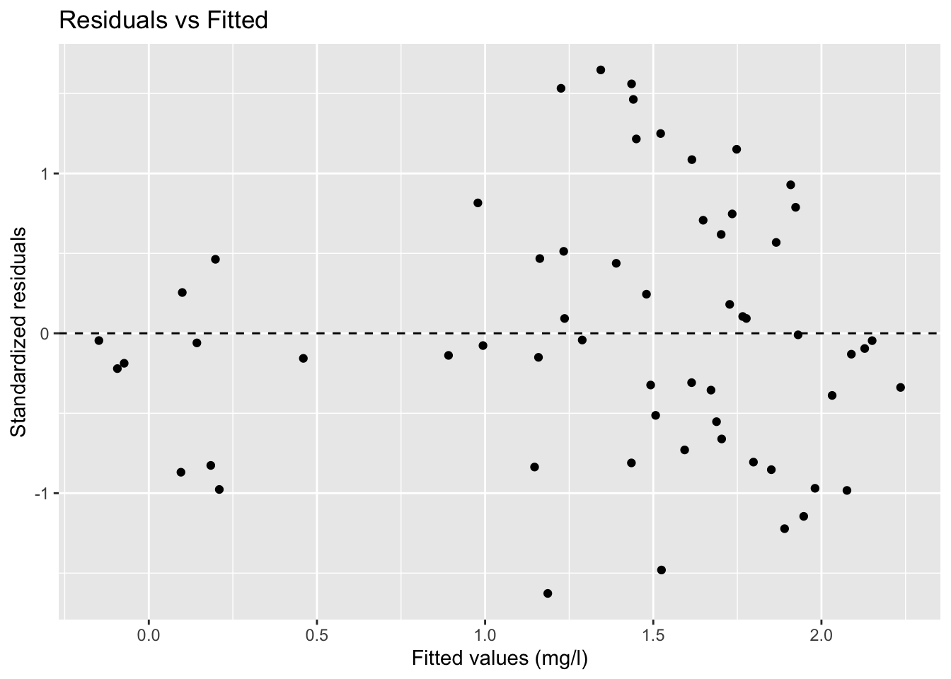
Look for:
- No systematic curvature
- No clear funnel shape
- Residuals spread roughly evenly around zero
As discussed earlier, a funnel shape suggests changing variance (heteroscedasticity), meaning the model errors become larger or smaller across the prediction range.
In mixed-effects modeling, we still want residual variability to remain reasonably stable after accounting for subject-level effects.
QQ Plot of Residuals
qqnorm(resid(lme_slope))
qqline(resid(lme_slope))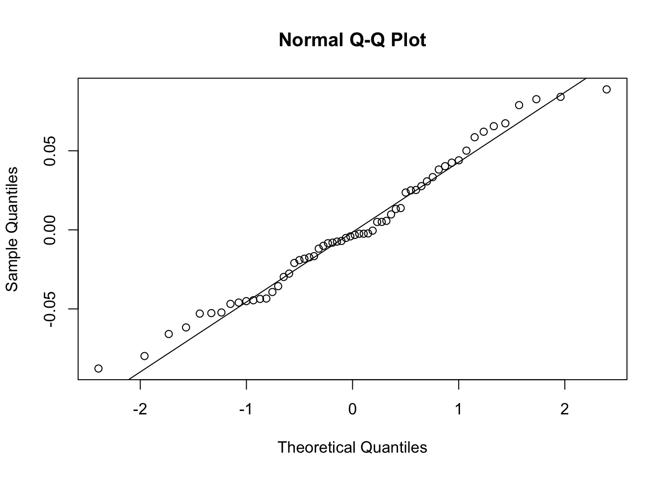
Assesses residual normality.
QQ Plot of Random Slopes
qqnorm(ranef(lme_slope)[, "Time"])
qqline(ranef(lme_slope)[, "Time"])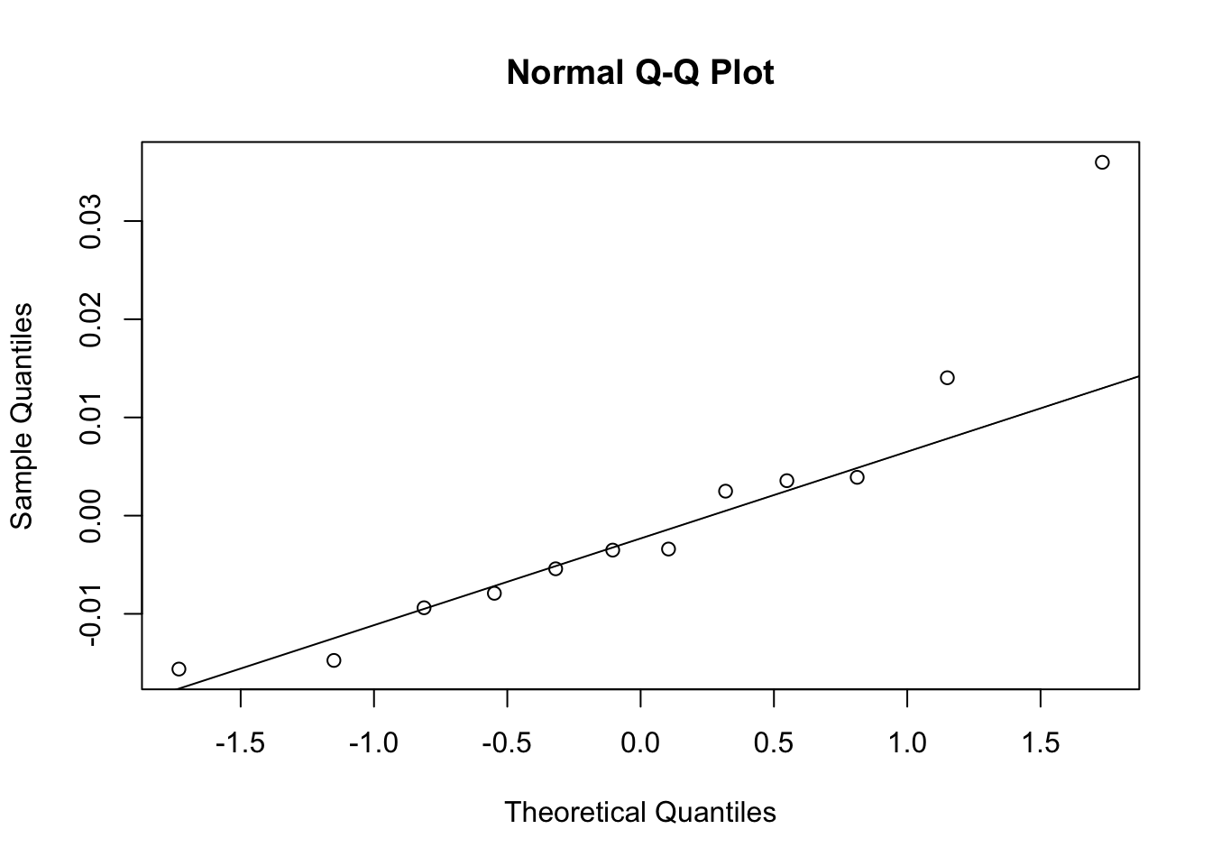
Assesses normality of subject-level elimination variability.
Extracting Components
fixef(lme_slope)(Intercept) Time
2.34455104 -0.08610951 ranef(lme_slope) %>% head() (Intercept) Time
6 -0.28299469 -0.003401271
7 -0.03098570 -0.003509436
8 -0.16352045 0.003902133
11 -0.19354278 -0.009380070
3 0.02347947 -0.007907807
2 0.01271365 -0.014743417VarCorr(lme_slope)Subject = pdLogChol(Time)
Variance StdDev Corr
(Intercept) 0.0384246349 0.19602203 (Intr)
Time 0.0002107216 0.01451625 -0.017
Residual 0.0029055459 0.05390312 These quantify:
- Population structure
- Subject deviations
- Variance components
Strategies
- Begin with visualization of subject-level trajectories.
- Fit pooled model for comparison.
- Fit random intercept model.
- Fit random intercept + slope model.
- Compare visually and statistically.
- Always examine diagnostics before drawing conclusions.
Common Mistakes
- Treating mixed-effects models as “just pooled regression with extra parameters”
- Confusing fixed effects with random effects
- Interpreting subject-specific predictions as population predictions
- Ignoring variability in slopes across subjects
- Assuming repeated measures are independent
- Trusting model output without checking diagnostics
- Forgetting that random effects can be correlated
- Focusing only on fit statistics instead of biological interpretation
Practice Problems
- Compare AIC of pooled and mixed models.
- Interpret random slope variance in PK terms.
- Explain shrinkage using the faceted plots.
- Identify one assumption diagnostics are checking.
TipStep-by-Step Solutions
Problem 1
AIC(lm_pooled)[1] 17.9586AIC(lme_slope)[1] -71.93471Problem 2
Random slope variance represents between-subject elimination variability.
Problem 3
Subject-specific curves are pulled toward the population mean when data are limited.
Problem 4
Normality and homoscedasticity of residuals; normality of random effects.
Summary
- Mixed-effects models model hierarchical PK data appropriately.
- Fixed effects represent population-average elimination.
- Random effects quantify biological variability.
- Conditional and marginal predictions differ fundamentally.
- Diagnostics are essential for responsible modeling.
TipQuick Tips
- Always compare pooled and hierarchical fits.
- Use faceting to understand variability.
- Check both residual and random-effect assumptions.
- Interpret parameters biologically before statistically.