library(tidyverse)
library(nlme)

data(Theoph)

one_comp_cl <- function(Time, dose, lka, lCL, lV) {
  ka <- exp(lka)
  CL <- exp(lCL)
  V  <- exp(lV)
  k  <- CL / V

  (dose * ka / (V * (ka - k))) * (exp(-k * Time) - exp(-ka * Time))
}

theoph_data <- Theoph %>%
rename(dose = Dose)Nonlinear Mixed-Effects Modeling with nlme()
One-Compartment Oral PK Model with Theoph
Learning Objectives
By the end of this lesson, you will be able to:
- Define a one-compartment oral PK model as an R function
- Explain the difference between \(k_e\) and clearance (CL), and why PMx often prefers CL
- Fit a nonlinear mixed-effects model using
nlme() - Interpret fixed and random effects in structural PK terms (CL, V, \(k_e\))
- Perform core diagnostics for nonlinear mixed-effects models
- Spot (and communicate) unit/scaling assumptions such as mg/kg dosing
Key Ideas
- Nonlinear mixed-effects models combine mechanistic structure with hierarchical variability.
- In PMx, clearance (CL) is often more interpretable and transferable than \(k_e\).
- \(k_e\) is a derived parameter: \(k_e = \frac{CL}{V}\).
- Parameterization matters: the same curve can be described with different parameters, but interpretation changes.
- Even “good-looking fits” require you to track units and assumptions.
Worked Example 1: The One-Compartment Oral Model
A one-compartment oral model with first-order absorption and elimination is:
\[ C(t) = \frac{F \cdot D \cdot k_a}{V (k_a - k)}\left(e^{-k t} - e^{-k_a t}\right), \quad \text{where } k = \frac{CL}{V}. \]
We will estimate:
- \(k_a\) : absorption rate constant
- \(CL\) : clearance
- \(V\) : volume
and compute the derived elimination rate:
\[ k_e = \frac{CL}{V}. \]
Tip
Why CL instead of \(k_e\)?
In PMx, CL is usually the parameter of interest for physiology, covariates, scaling, and simulation.
\(k_e\) can be convenient, but it mixes CL and V into one number, which can hide what is actually changing.
Worked Example 2: Units and Dose Scaling in Theoph
The Theoph dataset reports Dose in mg/kg.
That means:
- Dose can differ by subject
- Dose is already normalized by body size
If we plug Dose directly into the model, then parameters like V and CL are effectively estimated on a per-kg basis (e.g., L/kg and L/kg/h), which is internally consistent for this dataset.
Warning
If dose were in mg (not mg/kg), you would need to model body size explicitly (e.g., include weight/allometry) to keep units and interpretation consistent.
Worked Example 3: Define the Model Function (CL/V Parameterization)
We model parameters on the log scale to keep them positive:
- \(k_a = e^{\ell k_a}\)
- \(CL = e^{\ell CL}\)
- \(V = e^{\ell V}\)
Exponentiating the log-parameters guarantees that the resulting PK parameters remain positive during estimation.
This is important because negative values for \(k_a\), CL, or V are not biologically meaningful.
Worked Example 4: Fit a Nonlinear Mixed-Effects Model with nlme()
A practical first random-effects choice for PK is to allow variability in CL and V.
nlme_model <- nlme(
  conc ~ one_comp_cl(Time, dose, lka, lCL, lV),
  data = theoph_data,
  fixed  = lka + lCL + lV ~ 1,
  random = lCL + lV ~ 1 | Subject,
  start  = c(lka = log(1), lCL = log(0.04), lV = log(0.5))
)

summary(nlme_model)
Nonlinear mixed-effects model fit by maximum likelihood
Model: conc ~ one_comp_cl(Time, dose, lka, lCL, lV)
Data: theoph_data
AIC BIC logLik
436.7894 456.969 -211.3947
Random effects:
Formula: list(lCL ~ 1, lV ~ 1)
Level: Subject
Structure: General positive-definite, Log-Cholesky parametrization
StdDev Corr
lCL 0.2640696 lCL
lV 0.2052924 0.154
Residual 1.0194606
Fixed effects: lka + lCL + lV ~ 1
Value Std.Error DF t-value p-value
lka 0.419098 0.08184737 118 5.12048 0
lCL -3.235707 0.09290705 118 -34.82736 0
lV -0.761460 0.06918161 118 -11.00668 0
Correlation:
lka lCL
lCL -0.248
lV 0.368 -0.048
Standardized Within-Group Residuals:
Min Q1 Med Q3 Max
-2.1939119 -0.4550642 0.0000000 0.3090983 3.6855558
Number of Observations: 132
Number of Groups: 12 Here:
fixed = lka + lCL + lV ~ 1estimates one population-average value for each parameterrandom = lCL + lV ~ 1 | Subjectallows subjects to deviate from the population values for CL and V- Variability is modeled on the log scale
In this first model, we allow variability in CL and V but keep \(k_a\) fixed across subjects for simplicity and stability.
Interpretation:
- Fixed effects are population-average log-parameters
- Random effects describe subject deviations in CL and V (on the log scale)
Random-Effects Covariance Structure in nlme()
As in the previous mixed-effects lesson, random effects can be modeled with either:
- A full covariance structure (
pdSymm) - A diagonal covariance structure (
pdDiag)
By default:
random = lCL + lV ~ 1 | Subjectallows variability in both CL and V and also allows those random effects to be correlated.
You can inspect the estimated variance-covariance structure using:
VarCorr(nlme_model)Subject = pdLogChol(list(lCL ~ 1,lV ~ 1))
Variance StdDev Corr
lCL 0.06973277 0.2640696 lCL
lV 0.04214497 0.2052924 0.154
Residual 1.03929990 1.0194606 If you instead want to assume independent variability between CL and V, you can use a diagonal structure:
nlme_diag <- nlme(
  conc ~ one_comp_cl(Time, dose, lka, lCL, lV),
  data = theoph_data,
  fixed  = lka + lCL + lV ~ 1,
  random = pdDiag(lCL + lV ~ 1),
  groups = ~ Subject,
  start  = c(lka = log(1), lCL = log(0.04), lV = log(0.5))
)
In PK terms, this asks whether subjects with higher clearance also tend to have systematically different volumes.
Worked Example 5: Convert Fixed Effects Back to PK Parameters
fe <- fixef(nlme_model)

ka_pop <- exp(fe["lka"])
CL_pop <- exp(fe["lCL"])
V_pop  <- exp(fe["lV"])
ke_pop <- CL_pop / V_pop

tibble(
  ka_pop = ka_pop,
  CL_pop = CL_pop,
  V_pop  = V_pop,
  ke_pop = ke_pop,
  half_life_pop = log(2) / ke_pop
)
# A tibble: 1 × 5
ka_pop CL_pop V_pop ke_pop half_life_pop
<dbl> <dbl> <dbl> <dbl> <dbl>
1 1.52 0.0393 0.467 0.0842 8.23This is a nice teaching moment:
nlme()estimates CL and V- \(k_e\) and half-life are derived quantities
Worked Example 6: Visualize Individual vs Population Predictions
As in the previous mixed-effects lesson, we can compare:
- Subject-specific predictions (conditional)
- Population-average predictions (marginal)
In nlme, the easiest way to obtain these is:
fitted(nlme_model)→ subject-specific predictionspredict(nlme_model, level = 0)→ population predictions
theoph_data <- theoph_data %>%
  mutate(
    pred_individual = fitted(nlme_model),
    pred_population = predict(nlme_model, level = 0)
  )
Now overlay both on a faceted plot:
ggplot(theoph_data, aes(Time, conc)) +
  geom_point() +
  geom_line(aes(y = pred_individual, group = Subject)) +
  geom_line(aes(y = pred_population, group = Subject), linetype = 2) +
  facet_wrap(~ Subject) +
  labs(
    title = "Nonlinear Mixed-Effects Fit: Individual (solid) vs Population (dashed)",
    y = "Concentration"
  )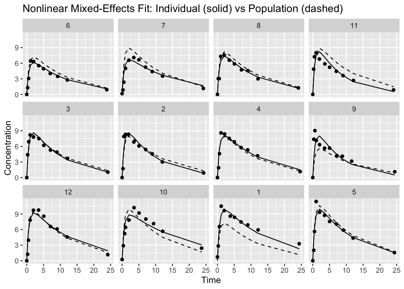
How to read this:
- The dashed curve is the same underlying population shape, evaluated at each subject’s dose and time points
- The solid curve shows how each subject deviates from that population curve via random effects
If the model is reasonable, the individual curves should track each subject’s profile without “over-chasing” noise, while the population curve provides a stable reference.
Diagnostics
1. Residuals vs Fitted
resid_vals <- resid(nlme_model, type = "pearson")

ggplot(
  data.frame(fitted = fitted(nlme_model), resid = resid_vals),
  aes(fitted, resid)
) +
  geom_point() +
  geom_hline(yintercept = 0, linetype = 2) +
  labs(title = "Residuals vs Fitted",
       x = "Fitted Values",
       y = "Pearson Residuals")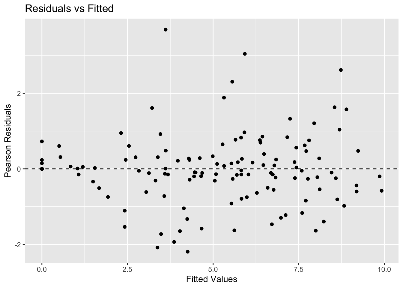
Look for:
- No obvious curvature (structure is adequate)
- Roughly constant spread (error model is plausible)
2. QQ Plot of Random Effects (CL)
qqnorm(ranef(nlme_model)[, "lCL"])
qqline(ranef(nlme_model)[, "lCL"])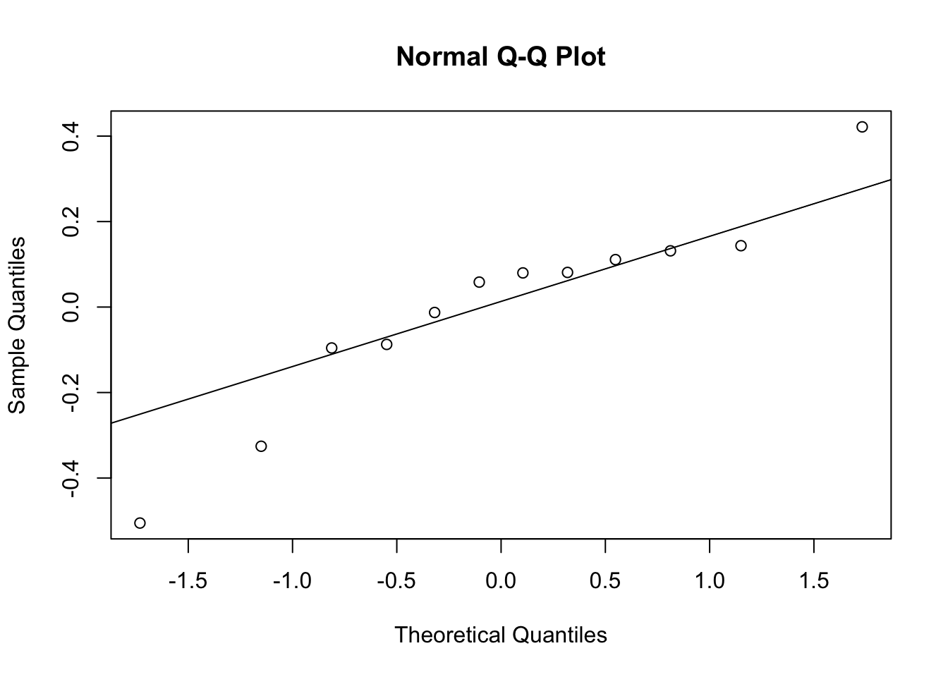
This checks the normality assumption of random effects (on the log scale).
Structural vs Hierarchical Comparison
Conceptually:
- Separate
nls()fits: each subject is isolated → unstable estimates, no population summary nlme(): population + individual deviations → borrowing strength + interpretable variability
This is the core idea behind population PK modeling.
Strategies
- Start with a clear structural model and parameter meanings.
- Prefer CL/V parameterization when teaching PMx thinking (CL is what we care about).
- Keep parameters positive by modeling them on the log scale.
- Add random effects gradually (start with CL and/or V).
- Always visualize fitted curves by subject.
Common Mistakes
- Confusing \(k_e\) with clearance (CL)
- Forgetting that \(k_e\) is derived from CL and V
- Ignoring units when interpreting CL and V
- Adding too many random effects too early
- Assuming a successful fit means the model is biologically correct
- Forgetting that random effects are modeled on the log scale
- Trusting population predictions without checking subject-level fits
- Ignoring implausible parameter estimates after fitting
Practice Problems
- Add random effects on \(k_a\) as well. What changes?
- Extract variance components and identify which parameter is most variable.
- Compute each subject’s implied \(k_e\) from their random effects (hint: subject CL and V).
- In one paragraph, explain why CL/V parameterization is preferable to modeling \(k_e\) directly in PMx work.
TipStep-by-Step Solutions
Problem 1
nlme_ka <- nlme(
  conc ~ one_comp_cl(Time, dose, lka, lCL, lV),
  data = theoph_data,
  fixed  = lka + lCL + lV ~ 1,
  random = lka + lCL + lV ~ 1 | Subject,
  start  = c(lka = log(1), lCL = log(0.04), lV = log(0.5))
)
If the fit becomes unstable, that is informative: you may not have enough information to estimate variability in \(k_a\) reliably from this dataset.
Problem 2
VarCorr(nlme_ka)Subject = pdLogChol(list(lka ~ 1,lCL ~ 1,lV ~ 1))
Variance StdDev Corr
lka 0.40669741 0.6377283 lka lCL
lCL 0.06309330 0.2511838 -0.089
lV 0.01477498 0.1215524 -0.197 0.994
Residual 0.46488727 0.6818264 Look at the estimated random-effect variances for lCL and lV.
The parameter with the larger variance shows greater between-subject variability on the log scale.
Problem 3
re <- ranef(nlme_ka) %>%
  rownames_to_column("Subject")

fe <- fixef(nlme_ka)

re %>%
  mutate(
    ka = exp(fe["lka"]),
    CL = exp(fe["lCL"] + lCL),
    V  = exp(fe["lV"]  + lV),
    ke = CL / V
  ) %>%
  select(Subject, CL, V, ke)
Subject CL V ke
1 6 0.04995676 0.5107577 0.09780914
2 7 0.04989074 0.5155802 0.09676622
3 8 0.04693208 0.4944255 0.09492244
4 11 0.05949112 0.5437188 0.10941524
5 3 0.04189983 0.4636412 0.09037125
6 2 0.04158710 0.4624081 0.08993593
7 4 0.03652038 0.4394642 0.08310206
8 9 0.03050002 0.3889358 0.07841916
9 12 0.03744340 0.4465899 0.08384291
10 10 0.03393042 0.4295828 0.07898460
11 1 0.02309517 0.3512610 0.06574933
12 5 0.04464058 0.4821363 0.09258912Because \(k_e = CL / V\), each subject’s elimination rate depends on both their individual CL and individual V.
Problem 4
CL links naturally to physiology, covariates, scaling, and simulation.
\(k_e\) is derived from CL and V, so changes in \(k_e\) can come from CL, V, or both. That makes it harder to interpret mechanistically than modeling CL and V directly.
Summary
- In PMx, CL and V are typically the core PK parameters; \(k_e\) is derived.
- Theoph uses dose in mg/kg, so CL and V are effectively per-kg parameters in this setup.
nlme()fits mechanistic structure while modeling between-subject variability.- Subject-specific fits and diagnostics are essential for trustworthiness.
- This workflow is a direct conceptual bridge to population PK tools and advanced PMx frameworks.
TipQuick Tips
- Prefer CL/V parameterization for interpretability.
- Model parameters on the log scale to keep them positive.
- Start with random effects on CL and V before adding \(k_a\).
- Always facet by subject when checking fits.
- Track units: dose scaling changes parameter interpretation.