library(tidyverse)
data(Theoph)

Theoph %>%
  ggplot(aes(Time, conc, group = Subject)) +
  geom_line(alpha = 0.4) +
  geom_point() +
  labs(title = "Theophylline Concentration–Time Profiles",
       x = "Time (h)", y = "Concentration")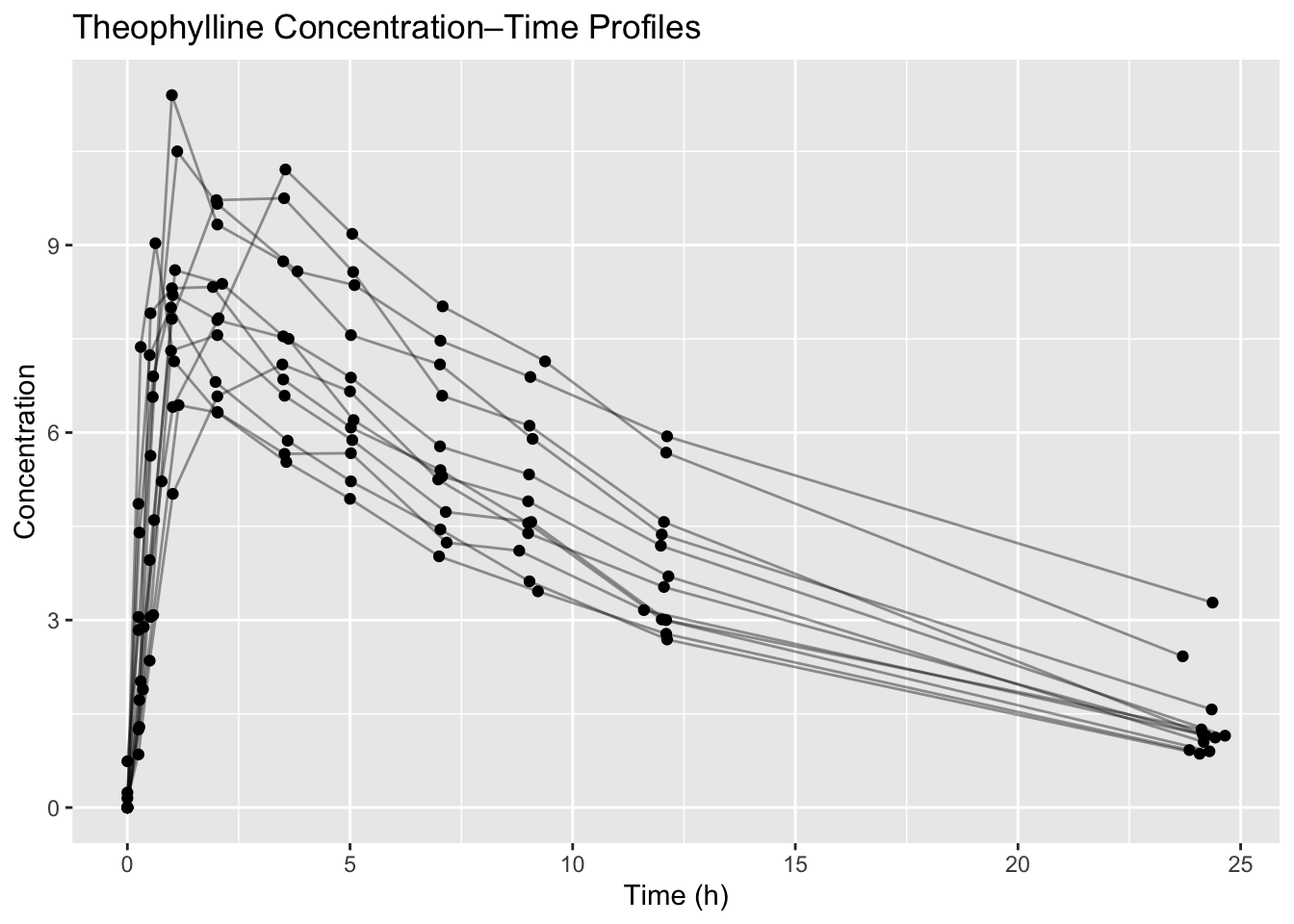
By the end of this lesson, you will be able to:
Modeling in pharmacometrics is not primarily about computing parameters.
It is about making assumptions explicit.
When you model, you are saying:
Exploratory models are:
They are not regulatory models. They are not population models.
They are structured questions written in mathematical form.
We begin with the classic Theoph dataset.
library(tidyverse)
data(Theoph)
Theoph %>%
ggplot(aes(Time, conc, group = Subject)) +
geom_line(alpha = 0.4) +
geom_point() +
labs(title = "Theophylline Concentration–Time Profiles",
x = "Time (h)", y = "Concentration")
Before modeling, pause.
Ask:
At this stage, you are already modeling — just without equations.
Suppose we ask:
Does concentration decline approximately exponentially after peak?
An exponential decline implies:
\[ C(t) = C_0 e^{-kt} \]
Taking logs:
\[ \log C(t) = \log C_0 - kt \]
This transforms the structural assumption into a linear relationship on the log scale.
terminal_data <- Theoph %>%
  filter(Time >= 4)

terminal_data %>%
  ggplot(aes(Time, log(conc), group = Subject)) +
  geom_line(alpha = 0.4) +
  geom_point() +
  labs(title = "Terminal Phase (Log Scale)",
       x = "Time (h)", y = "log(Concentration)")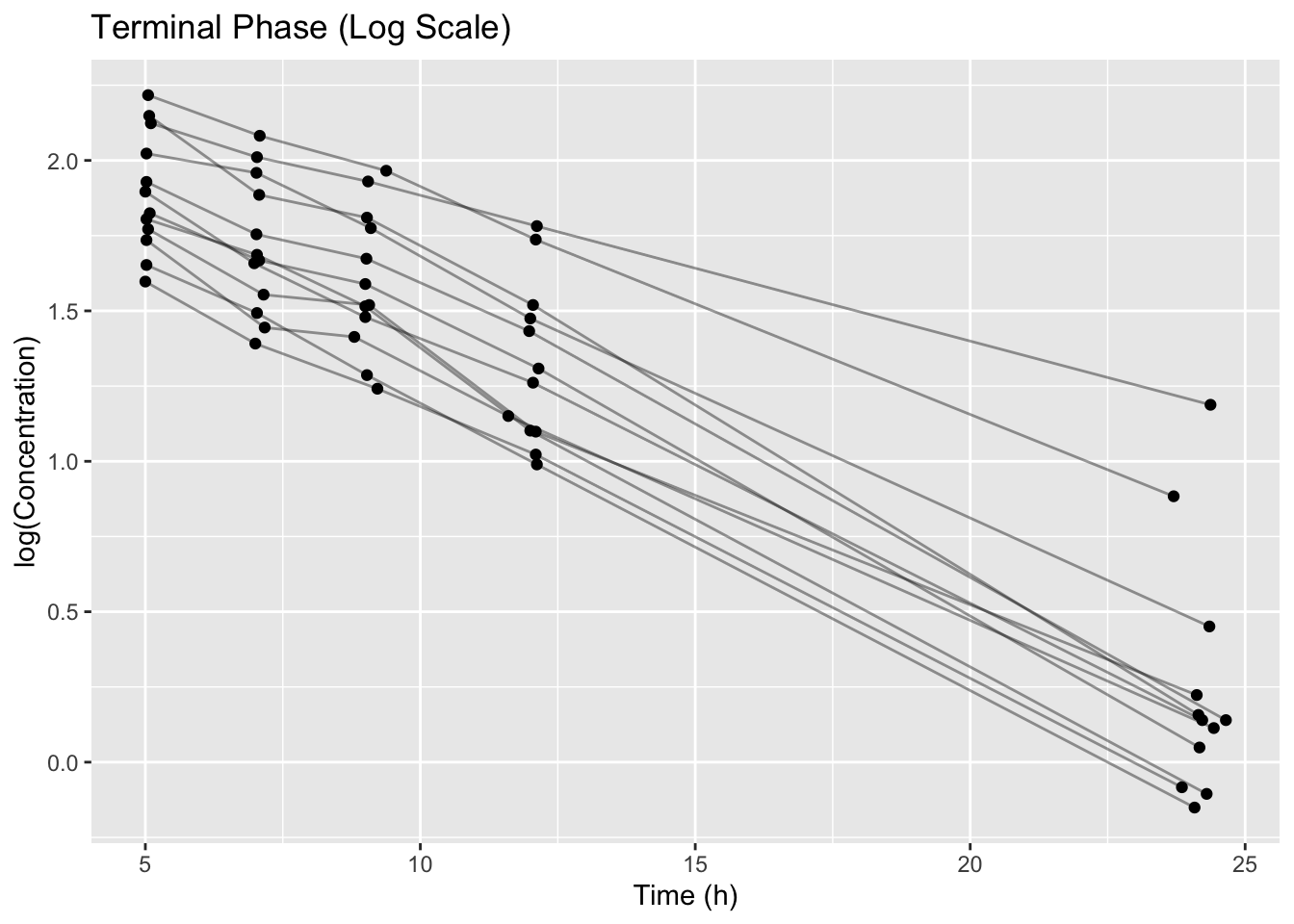
We are not estimating clearance formally.
We are testing whether a structural idea seems plausible.
Now we make the assumption explicit by fitting a linear model on the log scale.
\[ \log(C_{ij}) = \beta_0 + \beta_1 t_{ij} + \epsilon_{ij} \]
A naive pooled model:
This is often the first instinct in analysis — and it can be informative — but it is rarely realistic in pharmacometrics.
lm_pooled <- lm(log(conc) ~ Time, data = terminal_data)
summary(lm_pooled)
Call:
lm(formula = log(conc) ~ Time, data = terminal_data)

Residuals:
    Min      1Q  Median      3Q     Max
-0.4230 -0.1975 -0.0535  0.2047  0.9406

Coefficients:
             Estimate Std. Error t value Pr(>|t|)
(Intercept)  2.343802   0.069087   33.92   <2e-16 ***
Time        -0.086031   0.005185  -16.59   <2e-16 ***
---
Signif. codes:  0 '***' 0.001 '**' 0.01 '*' 0.05 '.' 0.1 ' ' 1

Residual standard error: 0.2719 on 58 degrees of freedom
Multiple R-squared:  0.826, Adjusted R-squared:  0.823
F-statistic: 275.3 on 1 and 58 DF,  p-value: < 2.2e-16
Interpret structurally:
Notice what the model does not account for: between-subject variability.
predict()A model becomes meaningful when we compare it to the data.
terminal_data <- terminal_data %>%
  mutate(pred_log = predict(lm_pooled))

ggplot(terminal_data, aes(Time, log(conc), group = Subject)) +
  geom_point() +
  geom_line(aes(y = pred_log)) +
  labs(title = "Observed vs Pooled Log-Linear Fit")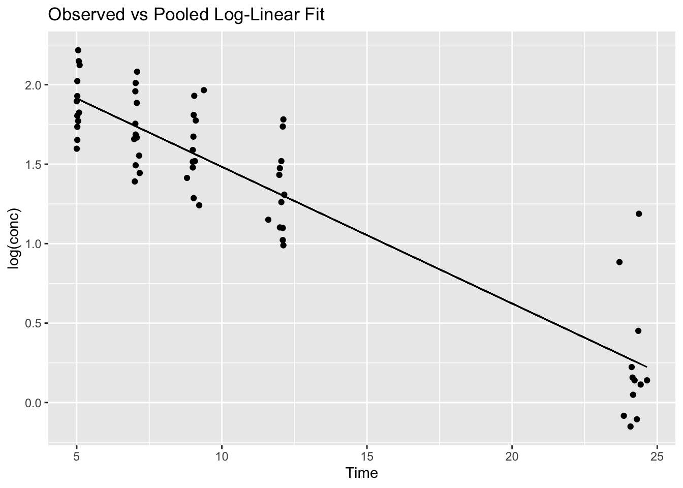
Ask:
This is the beginning of model criticism.
We will formalize diagnostic reasoning in the next lesson.
Exploratory models:
Confirmatory models:
A common mistake in PMx is treating an exploratory model as if it were a final population model.
Problem 1
Theoph %>%
  filter(Time < 2) %>%
  ggplot(aes(Time, conc, group = Subject)) +
  geom_line(alpha = 0.4) +
  geom_point()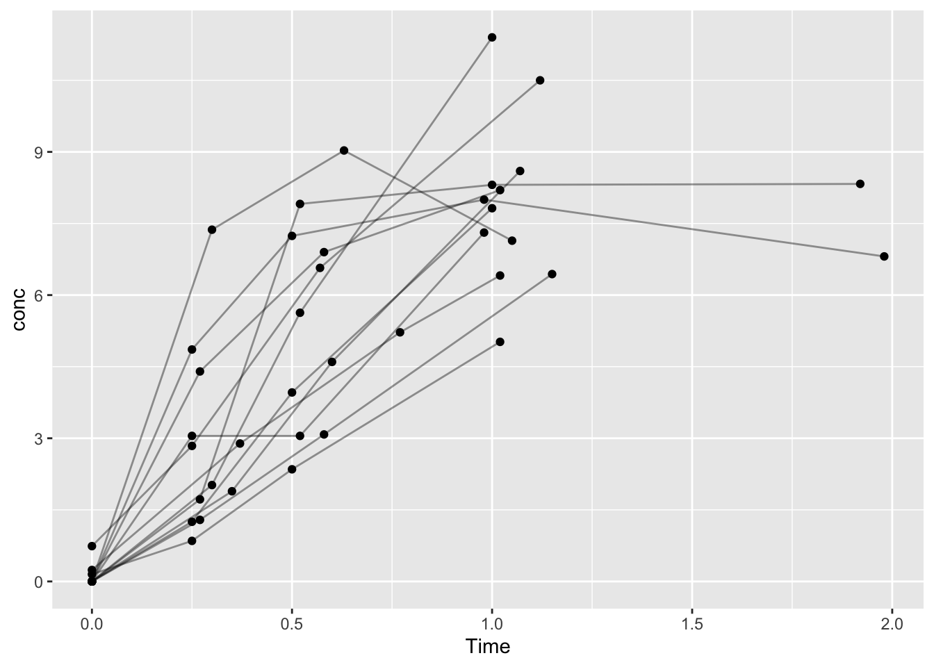
Early time points reflect absorption dynamics rather than simple elimination.
Problem 2
lm_linear <- lm(conc ~ Time, data = terminal_data)
summary(lm_linear)
Call:
lm(formula = conc ~ Time, data = terminal_data)

Residuals:
    Min      1Q  Median      3Q     Max
-1.7364 -0.8468 -0.1718  0.7396  2.9051

Coefficients:
            Estimate Std. Error t value Pr(>|t|)
(Intercept)  7.61771    0.30335   25.11   <2e-16 ***
Time        -0.26591    0.02277  -11.68   <2e-16 ***
---
Signif. codes:  0 '***' 0.001 '**' 0.01 '*' 0.05 '.' 0.1 ' ' 1

Residual standard error: 1.194 on 58 degrees of freedom
Multiple R-squared:  0.7017,    Adjusted R-squared:  0.6965
F-statistic: 136.4 on 1 and 58 DF,  p-value: < 2.2e-16
The linear-scale model typically misrepresents exponential decay.
Problem 3
Pooling assumes identical elimination rates across subjects and ignores hierarchical variability.