library(dplyr)
library(readr)
library(here)
library(nlme)
library(ggplot2)
library(MASS)
library(purrr)
library(tidyr)

resultspath <- here("courses", "foundations-r", "results", "modeling", "population")

nlme_path <- file.path(resultspath, "nlme_fit.rds")

if (!file.exists(nlme_path)) {
  stop("Frozen model not found. Run the previous lesson first.")
}

nlme_fit <- readRDS(nlme_path)Simulation & Scenario Exploration
Use the frozen nlme population model to simulate new dosing regimens, generate variability envelopes, and compute exposure metrics for decision-oriented interpretation.
Tip
Big picture: A fitted model is not the end — it is a tool.
In this lesson, we use the frozen population model to simulate new dosing scenarios and explore exposure metrics.
Learning Objectives
By the end of this lesson, you will be able to:
- Load a frozen
nlmemodel object reproducibly. - Simulate deterministic population predictions for new doses.
- Simulate stochastic profiles including inter-individual variability (IIV).
- Compute exposure metrics (Cmax, AUC).
- Visualize median and percentile envelopes.
- Interpret simulation results in a decision-oriented context.
Key Ideas
- Estimation and simulation are separate steps.
- Simulation uses fixed effects (and optionally variability).
- New doses can be explored without re-fitting the model.
- Extrapolation must be interpreted cautiously.
- Simulation supports decisions — it does not replace judgment.
Setup
Worked Example 1: Extract Population Parameters
First, we extract the fixed effects and convert them back to natural-scale PK parameters for simulation.
fe <- fixef(nlme_fit)

ka_pop <- exp(fe["lka"])
CL_pop <- exp(fe["lCL"])
V_pop  <- exp(fe["lV"])
Define structural function:
one_comp <- function(time, dose, ka, CL, V) {
  k <- CL / V
  (dose * ka / (V * (ka - k))) *
    (exp(-k * time) - exp(-ka * time))
}
Worked Example 2: Deterministic Simulation (Fixed Effects Only)
Simulate across doses, including a new 200 mg scenario.
time_grid <- seq(0, 24, by = 0.1)
dose_grid <- c(25, 50, 100, 200)

sim_det <- expand.grid(
  TIME = time_grid,
  DOSE = dose_grid
) %>%
  mutate(
    CONC = one_comp(TIME, DOSE, ka_pop, CL_pop, V_pop)
  )
Plot:
p_det <- ggplot(sim_det, aes(TIME, CONC, color = factor(DOSE))) +
  geom_line() +
  labs(
    title = "Deterministic Population Simulation",
    x = "Time (h)",
    y = "Concentration",
    color = "Dose (mg)"
  )

p_det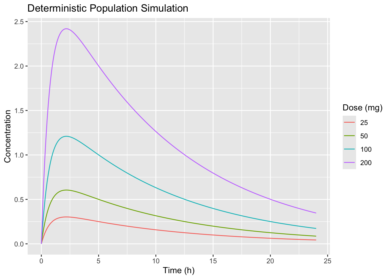
Worked Example 3: Stochastic Simulation (Add IIV)
Deterministic simulations use fixed effects only.
To visualize variability, we sample random effects and generate a distribution of profiles.
Step 1: Build an IIV covariance matrix
For simplicity, we’ll assume CL and V random effects are independent here (diagonal covariance).
vc <- VarCorr(nlme_fit)

omega2_CL <- as.numeric(vc["lCL", "Variance"])
omega2_V  <- as.numeric(vc["lV", "Variance"])

Sigma <- matrix(c(omega2_CL, 0,
                  0, omega2_V), nrow = 2)
Sigma
[,1] [,2]
[1,] 0.0192418 0.00000000
[2,] 0.0000000 0.08851451Step 2: Sample ETAs per virtual subject, then expand across the time grid
This avoids group_modify() size-mismatch pitfalls and makes the simulation flow explicit.
set.seed(20260226)

n_sim <- 200

# one row per simulated subject per dose
eta_tbl <- tidyr::crossing(
  DOSE = dose_grid,
  ID = 1:n_sim
) %>%
  mutate(
    eta = purrr::map(1:n(), ~ MASS::mvrnorm(1, mu = c(0, 0), Sigma = Sigma)),
    ETA_CL = purrr::map_dbl(eta, 1),
    ETA_V  = purrr::map_dbl(eta, 2)
  ) %>%
  dplyr::select(-eta)

eta_tbl %>% slice_head(n = 5)
# A tibble: 5 × 4
DOSE ID ETA_CL ETA_V
<dbl> <int> <dbl> <dbl>
1 25 1 0.146 -0.357
2 25 2 0.136 -0.0791
3 25 3 -0.139 0.463
4 25 4 -0.0562 0.0278
5 25 5 -0.111 0.250 Expand to a dense time grid and compute concentration:
sim_stoch <- tidyr::crossing(
  eta_tbl,
  TIME = time_grid
) %>%
  mutate(
    CL_i = exp(fe["lCL"] + ETA_CL),
    V_i  = exp(fe["lV"]  + ETA_V),
    ka_i = exp(fe["lka"]),
    CONC = one_comp(TIME, DOSE, ka_i, CL_i, V_i)
  ) %>%
  dplyr::select(DOSE, ID, TIME, CONC)

sim_stoch %>% slice_head(n = 5)
# A tibble: 5 × 4
DOSE ID TIME CONC
<dbl> <int> <dbl> <dbl>
1 25 1 0 0
2 25 1 0.1 0.0643
3 25 1 0.2 0.120
4 25 1 0.3 0.167
5 25 1 0.4 0.208 Step 3: Summarize percentile envelopes
sim_summary <- sim_stoch %>%
  group_by(DOSE, TIME) %>%
  summarise(
    p5  = quantile(CONC, 0.05),
    p50 = quantile(CONC, 0.50),
    p95 = quantile(CONC, 0.95),
    .groups = "drop"
  )
Plot the envelope (median + 5–95% band):
p_env <- ggplot(sim_summary, aes(TIME, p50, color = factor(DOSE))) +
  geom_line() +
  geom_ribbon(
    aes(ymin = p5, ymax = p95, fill = factor(DOSE)),
    alpha = 0.2,
    color = NA
  ) +
  labs(
    title = "Stochastic Simulation with IIV (Median + 5–95%)",
    x = "Time (h)",
    y = "Concentration",
    color = "Dose",
    fill = "Dose"
  )

p_env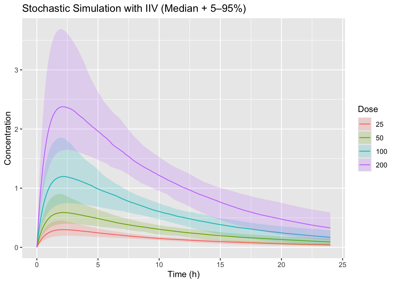
Worked Example 4: Exposure Metrics (Cmax, AUC0-24)
Compute exposure metrics per simulated subject.
calc_auc <- function(time, conc) {
  sum(diff(time) * (head(conc, -1) + tail(conc, -1)) / 2)
}

exposure <- sim_stoch %>%
  group_by(DOSE, ID) %>%
  summarise(
    Cmax = max(CONC),
    AUC0_24 = calc_auc(TIME, CONC),
    .groups = "drop"
  )

exposure %>%
  group_by(DOSE) %>%
  summarise(
    median_Cmax = median(Cmax),
    median_AUC = median(AUC0_24),
    .groups = "drop"
  )
# A tibble: 4 × 3
DOSE median_Cmax median_AUC
<dbl> <dbl> <dbl>
1 25 0.298 3.44
2 50 0.589 6.89
3 100 1.20 14.1
4 200 2.38 27.3
Warning
- Extrapolated doses (e.g., 200 mg) rely entirely on model assumptions.
- Structural misspecification propagates into simulation.
- Simulation results are conditional on estimated variability.
- Always state assumptions when presenting simulated results.
Strategies
- Load the frozen model using
readRDS(). - Use fixed effects for deterministic simulation.
- Sample random effects for variability simulation.
- Simulate over a dense time grid.
- Always visualize median and percentile bands.
- Compute exposure metrics systematically.
Common Mistakes
- Re-fitting the model inside the simulation workflow.
- Presenting deterministic curves as if they include population variability.
- Sampling random effects with the wrong variance scale.
- Comparing exposure metrics computed on different time grids.
- Treating extrapolated dose scenarios as confirmed observations.
Practice Problems
- Add a 300 mg scenario and compare deterministic exposure scaling.
- Add 300 mg to the stochastic simulation and summarize the variability envelope.
- Compare deterministic vs stochastic Cmax.
- Plot exposure vs dose using median AUC.
TipStep-by-Step Solutions
Problem 1: Add a 300 mg scenario and compare deterministic exposure scaling
First, extend the dose grid to include 300 mg.
dose_grid_ext <- c(25, 50, 100, 200, 300)Create deterministic simulations for the extended dose range.
sim_det_ext <- expand.grid(
  TIME = time_grid,
  DOSE = dose_grid_ext
) %>%
  mutate(
    CONC = one_comp(TIME, DOSE, ka_pop, CL_pop, V_pop)
  )
Compute deterministic exposure metrics.
det_exposure_ext <- sim_det_ext %>%
  group_by(DOSE) %>%
  summarise(
    Cmax = max(CONC),
    AUC0_24 = calc_auc(TIME, CONC),
    .groups = "drop"
  ) %>%
  mutate(
    dose_ratio_to_100 = DOSE / 100,
    auc_ratio_to_100 = AUC0_24 / AUC0_24[DOSE == 100],
    cmax_ratio_to_100 = Cmax / Cmax[DOSE == 100]
  )

det_exposure_ext
# A tibble: 5 × 6
DOSE Cmax AUC0_24 dose_ratio_to_100 auc_ratio_to_100 cmax_ratio_to_100
<dbl> <dbl> <dbl> <dbl> <dbl> <dbl>
1 25 0.302 3.53 0.25 0.25 0.25
2 50 0.605 7.07 0.5 0.5 0.5
3 100 1.21 14.1 1 1 1
4 200 2.42 28.3 2 2 2
5 300 3.63 42.4 3 3 3 For a linear one-compartment model, exposure should scale approximately proportionally with dose.
Problem 2: Add 300 mg to the stochastic simulation and summarize the variability envelope
Create a new random-effects table using the extended dose grid.
set.seed(20260226)

eta_tbl_ext <- tidyr::crossing(
  DOSE = dose_grid_ext,
  ID = 1:n_sim
) %>%
  mutate(
    eta = purrr::map(1:n(), ~ MASS::mvrnorm(1, mu = c(0, 0), Sigma = Sigma)),
    ETA_CL = purrr::map_dbl(eta, 1),
    ETA_V  = purrr::map_dbl(eta, 2)
  ) %>%
  dplyr::select(-eta)
Generate stochastic profiles for all doses, including 300 mg.
sim_stoch_ext <- tidyr::crossing(
  eta_tbl_ext,
  TIME = time_grid
) %>%
  mutate(
    CL_i = exp(fe["lCL"] + ETA_CL),
    V_i  = exp(fe["lV"]  + ETA_V),
    ka_i = exp(fe["lka"]),
    CONC = one_comp(TIME, DOSE, ka_i, CL_i, V_i)
  ) %>%
  dplyr::select(DOSE, ID, TIME, CONC)
Summarize the median and 5th–95th percentile envelope.
sim_summary_ext <- sim_stoch_ext %>%
  group_by(DOSE, TIME) %>%
  summarise(
    p5  = quantile(CONC, 0.05),
    p50 = quantile(CONC, 0.50),
    p95 = quantile(CONC, 0.95),
    .groups = "drop"
  )

sim_summary_ext %>% slice_head(n = 10)
# A tibble: 10 × 5
DOSE TIME p5 p50 p95
<dbl> <dbl> <dbl> <dbl> <dbl>
1 25 0 0 0 0
2 25 0.1 0.0278 0.0442 0.0714
3 25 0.2 0.0521 0.0825 0.133
4 25 0.3 0.0733 0.116 0.186
5 25 0.4 0.0917 0.145 0.232
6 25 0.5 0.108 0.169 0.270
7 25 0.6 0.121 0.191 0.304
8 25 0.7 0.133 0.209 0.332
9 25 0.8 0.144 0.225 0.356
10 25 0.9 0.153 0.239 0.376 Plot the extended variability envelope.
p_env_ext <- ggplot(sim_summary_ext, aes(TIME, p50, color = factor(DOSE))) +
  geom_line() +
  geom_ribbon(
    aes(ymin = p5, ymax = p95, fill = factor(DOSE)),
    alpha = 0.2,
    color = NA
  ) +
  labs(
    title = "Stochastic Simulation with IIV Including 300 mg",
    x = "Time (h)",
    y = "Concentration",
    color = "Dose",
    fill = "Dose"
  )

p_env_ext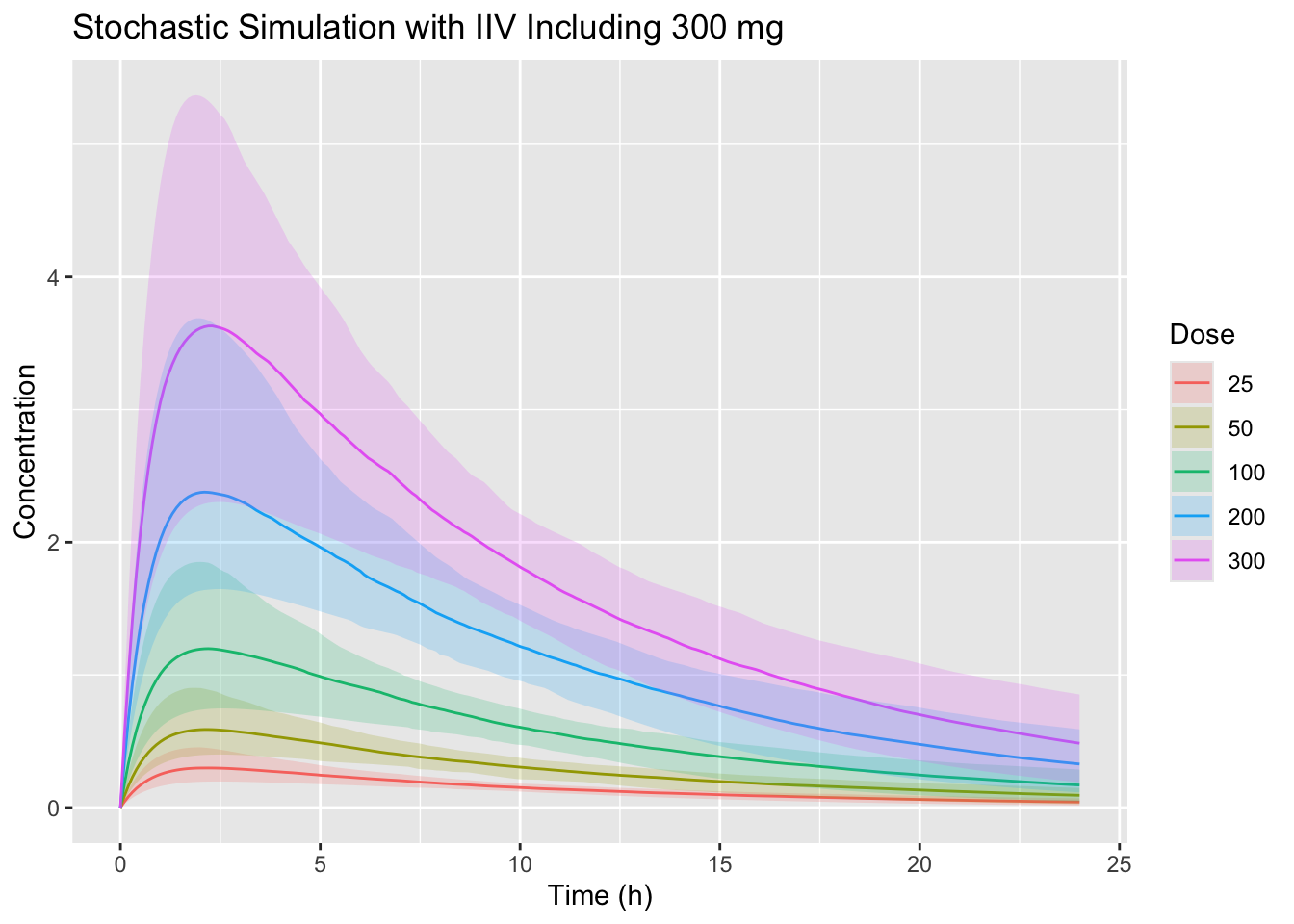
Problem 3: Compare deterministic vs stochastic Cmax
Compute deterministic Cmax from the fixed-effects simulation.
det_cmax <- sim_det %>%
  group_by(DOSE) %>%
  summarise(
    deterministic_Cmax = max(CONC),
    .groups = "drop"
  )
Compute stochastic Cmax summaries from the simulated-subject exposure table.
stoch_cmax <- exposure %>%
  group_by(DOSE) %>%
  summarise(
    median_stochastic_Cmax = median(Cmax),
    p5_stochastic_Cmax = quantile(Cmax, 0.05),
    p95_stochastic_Cmax = quantile(Cmax, 0.95),
    .groups = "drop"
  )
Join the results.
cmax_compare <- det_cmax %>%
  left_join(stoch_cmax, by = "DOSE")

cmax_compare
# A tibble: 4 × 5
DOSE deterministic_Cmax median_stochastic_Cmax p5_stochastic_Cmax
<dbl> <dbl> <dbl> <dbl>
1 25 0.302 0.298 0.196
2 50 0.605 0.589 0.400
3 100 1.21 1.20 0.747
4 200 2.42 2.38 1.65
# ℹ 1 more variable: p95_stochastic_Cmax <dbl>The deterministic value represents the fixed-effects subject, while the stochastic summaries reflect variability across virtual subjects.
Problem 4: Plot exposure vs dose using median AUC
Summarize AUC by dose.
auc_by_dose <- exposure %>%
  group_by(DOSE) %>%
  summarise(
    median_AUC = median(AUC0_24),
    p5_AUC = quantile(AUC0_24, 0.05),
    p95_AUC = quantile(AUC0_24, 0.95),
    .groups = "drop"
  )

auc_by_dose
# A tibble: 4 × 4
DOSE median_AUC p5_AUC p95_AUC
<dbl> <dbl> <dbl> <dbl>
1 25 3.44 2.78 4.16
2 50 6.89 5.49 8.48
3 100 14.1 11.0 17.0
4 200 27.3 22.4 35.0 Plot median AUC versus dose.
p_auc <- ggplot(auc_by_dose, aes(DOSE, median_AUC)) +
  geom_point(size = 2) +
  geom_line() +
  geom_errorbar(aes(ymin = p5_AUC, ymax = p95_AUC), width = 5) +
  labs(
    title = "Exposure vs Dose",
    subtitle = "Median AUC with 5th–95th percentile interval",
    x = "Dose",
    y = "AUC0-24"
  )

p_auc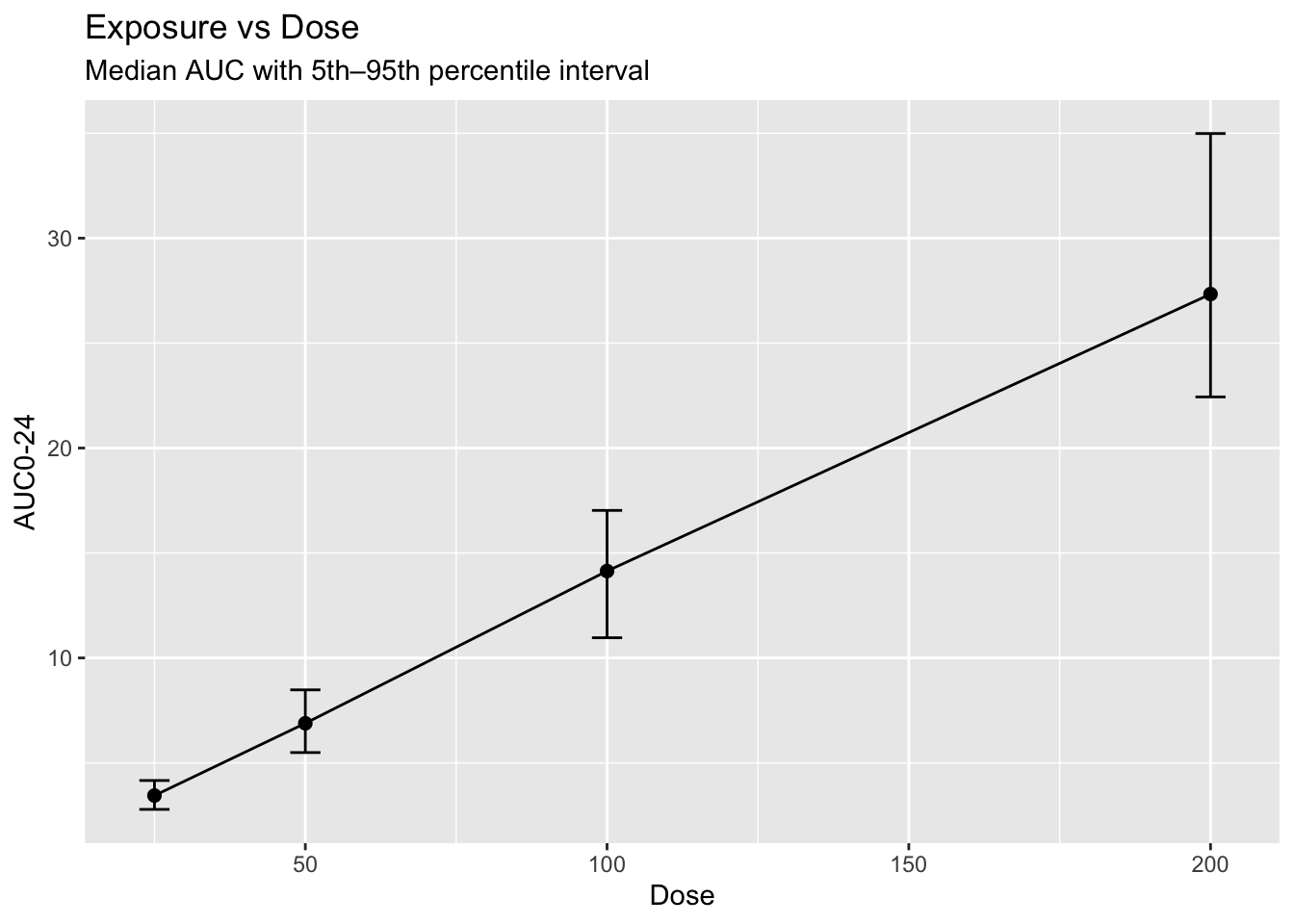
Save the plot.
ggsave(file.path(resultspath, "exposure_vs_dose_auc.png"), p_auc, width = 7, height = 5)Summary
- You loaded a frozen population model.
- You simulated deterministic and stochastic scenarios.
- You visualized variability envelopes.
- You computed exposure metrics.
- You explored extrapolated dose scenarios.
- You completed the full workflow: raw data → model → simulation → interpretation.
TipQuick Tips
- Always freeze models before simulation.
- Separate deterministic and stochastic simulation clearly.
- Use percentile bands for communication clarity.
- Exposure metrics drive decisions more than curves alone.
- State assumptions explicitly when presenting simulation results.