library(tidyverse)

data(Theoph, package = "datasets")

theoph <- Theoph %>%
  rename(
    ID   = Subject,
    TIME = Time,
    DV   = conc
  ) %>%
arrange(ID, TIME)Summaries, Variability, and Overplotting
Use summary layers responsibly and learn how to scale visualization strategies when PK datasets become large.
Tip
Core idea of this lesson: When N is small, individuals dominate.
When N is large, structure disappears.
Summary layers and density strategies are tools for responsible compression — not shortcuts.
Learning Objectives
By the end of this lesson, you will be able to:
- Define nominal time using a protocol schedule and align observations before summarizing.
- Compute mean and variability summaries correctly.
- Recognize what summary layers hide.
- Detect overplotting in large datasets.
- Use alpha blending, sampling, binning, and summaries strategically.
- Combine individuals and summaries without losing interpretability.
Key Ideas
- Summary layers compress data and always hide individual variability.
- Time alignment (e.g., nominal time) is required before computing meaningful summaries.
- Large datasets introduce overplotting, which obscures structure.
- Visualization strategies (alpha, sampling, summaries) are tools for controlled compression.
- Additive summaries (mean ± SD) and multiplicative summaries (log-scale) describe different types of variability.
- Individual-level structure should remain visible somewhere in the analysis workflow.
Part I — Responsible Summaries (Theoph)
Why Alignment Comes First
When computing:
group_by(TIME) %>% summarise(mean(DV))you assume subjects were sampled at identical times.
In real studies:
- Sampling times may deviate slightly.
- Sparse designs are common.
- Raw-time averaging may mix non-comparable observations.
Note
Summary curves are only valid after defining aligned (nominal) time. Study protocols usually define nominal sampling times.
Setup (Theoph)
Protocol schedule:
nominal_times <- c(0, 0.25, 0.5, 1, 2, 3.5, 5, 7, 9, 12, 24)
nominal_times
[1] 0.00 0.25 0.50 1.00 2.00 3.50 5.00 7.00 9.00 12.00 24.00Create Nominal-Time Bins
midpoints <- (nominal_times[-1] + nominal_times[-length(nominal_times)]) / 2
breaks <- c(-Inf, midpoints, Inf)

theoph <- theoph %>%
  mutate(
    NOM_TIME = cut(
      TIME,
      breaks = breaks,
      labels = nominal_times,
      include.lowest = TRUE,
      right = TRUE
    ),
    NOM_TIME = as.numeric(as.character(NOM_TIME))
  )
Compute Summary Statistics
summary_df <- theoph %>%
  group_by(NOM_TIME) %>%
  summarise(
    mean_DV = mean(DV),
    sd_DV   = sd(DV),
    n       = n(),
    .groups = "drop"
  ) %>%
  arrange(NOM_TIME)
Worked Example 1: Individuals + Mean
ggplot() +
  geom_line(data = theoph,
            aes(TIME, DV, group = ID),
            alpha = 0.25, color = "grey60") +
  geom_line(data = summary_df,
            aes(NOM_TIME, mean_DV),
            linewidth = 1) +
  labs(
    title = "Individuals + Mean Summary",
    x = "Time (hours)",
    y = "Concentration"
  ) +
  theme_minimal()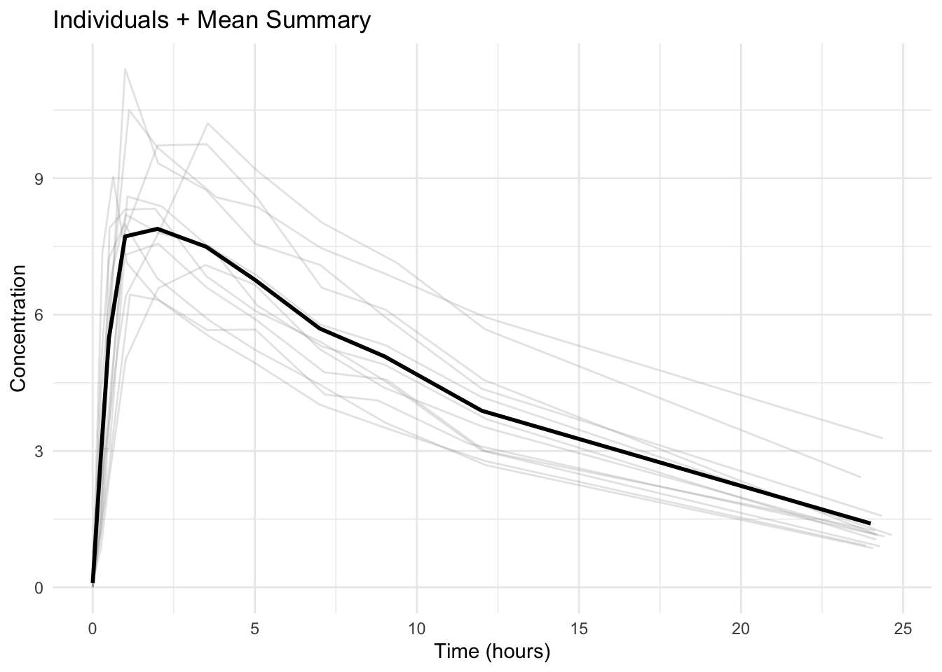
Warning
The mean hides heterogeneity.
Always inspect individuals somewhere in your workflow.
Worked Example 2: Variability Ribbon
ggplot(summary_df, aes(NOM_TIME, mean_DV)) +
  geom_line(linewidth = 1) +
  geom_ribbon(aes(ymin = mean_DV - sd_DV,
                  ymax = mean_DV + sd_DV),
              alpha = 0.2) +
  labs(
    title = "Mean ± SD by Nominal Time",
    x = "Nominal Time (hours)",
    y = "Concentration"
  ) +
  theme_minimal()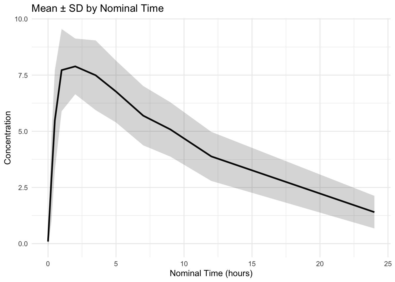
Note
PK variability is often multiplicative.
Log-scale summaries may be more appropriate in some settings.
Note
When combining individuals and summaries, it helps to make layers visually distinct.
Common choices include using a thicker line for the summary (linewidth) or a different linetype (e.g., dashed) so readers immediately know what is “individual” vs “population summary.”
Part II — Scaling Up: Overplotting (Remifentanil)
When N increases, individual profiles overlap heavily and structure disappears.
Setup (Remifentanil)
library(nlme)

data(Remifentanil, package = "nlme")

remi <- as_tibble(Remifentanil) %>%
  rename(
    ID   = ID,
    TIME = Time,
    DV   = conc
  ) %>%
  filter(!is.na(DV)) %>%
  arrange(ID, TIME)
A Note on Nominal Time for Remifentanil
Unlike Theoph, the Remifentanil dataset contains many observed sampling times that are close to a study schedule (e.g., 20.00, 20.05, 20.57, 21.08).
For summaries (median/IQR, ribbons, etc.), it’s often better to align times to protocol nominal times first.
Below is a reasonable teaching approximation of the protocol schedule based on the observed Time values you saw:
nominal_times_remi <- c(
  0,1.5,2,2.5,3,3.5,4,4.5,5,6,7,8,9,10,12,14,16,18,
  20,20.05,20.5,21,21.5,22,22.5,23,23.5,24,24.5,25,
  26,28,29,30,32,34,36,38,40,45,50,55,60,65,70,
  80,90,100,110,120,140,170,200,230
)

# Convert observed TIME to nominal bins using midpoint boundaries
midpoints_remi <- (nominal_times_remi[-1] + nominal_times_remi[-length(nominal_times_remi)]) / 2
breaks_remi <- c(-Inf, midpoints_remi, Inf)

remi <- remi %>%
  mutate(
    NOM_TIME = cut(
      TIME,
      breaks = breaks_remi,
      labels = nominal_times_remi,
      include.lowest = TRUE,
      right = TRUE
    ),
    NOM_TIME = as.numeric(as.character(NOM_TIME))
  )
Note
Teaching moment: In real projects, you should get nominal times from the protocol (or the data collection plan), then align observations to those nominal times before summarizing.
Worked Example 3: Overplotting Problem
ggplot(remi, aes(TIME, DV, group = ID)) +
  geom_line() +
  scale_y_log10() +
  labs(title = "Large Dataset: Overplotting") +
  theme_minimal()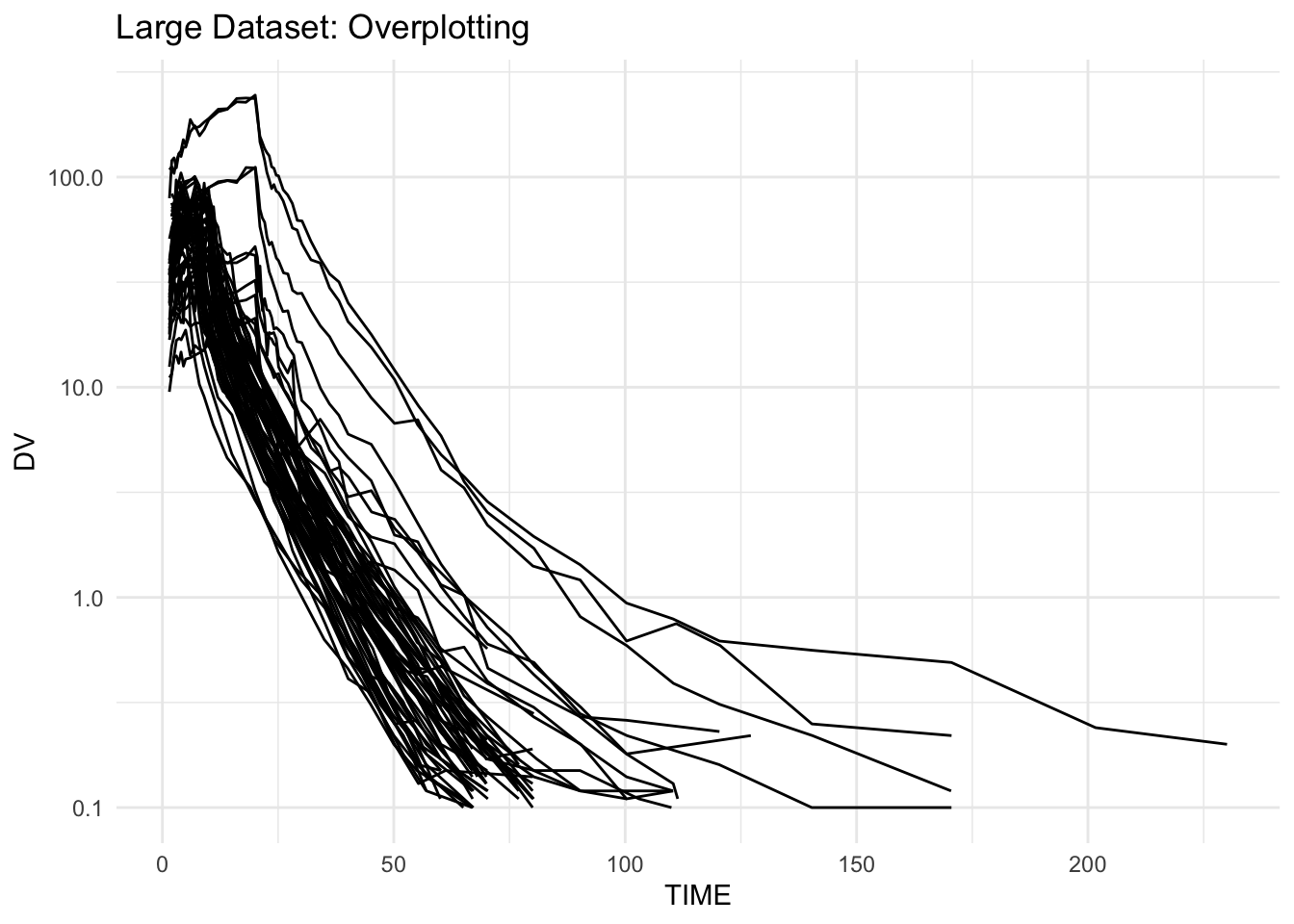
Unreadable “spaghetti” is a visualization problem.
Strategy 1: Alpha Blending
ggplot(remi, aes(TIME, DV, group = ID)) +
  geom_line(alpha = 0.1, color = "grey40") +
  scale_y_log10() +
  labs(title = "Alpha Blending Reveals Density") +
  theme_minimal()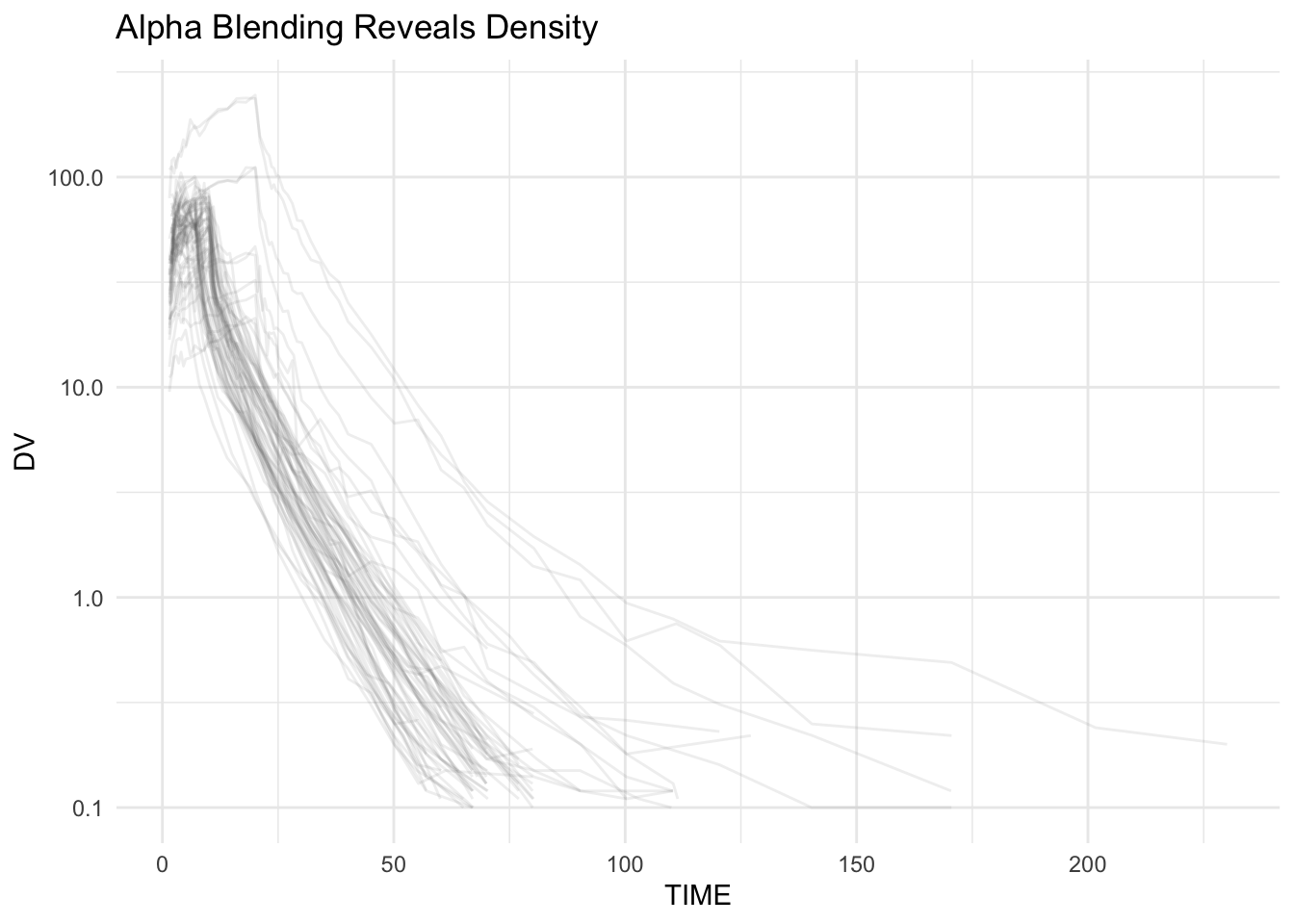
Dense regions appear darker.
Strategy 2: Sampling (Use Carefully)
set.seed(123)
sample_ids <- sample(unique(remi$ID), 20)

ggplot(remi %>% filter(ID %in% sample_ids),
       aes(TIME, DV, group = ID)) +
  geom_line(alpha = 0.6) +
  scale_y_log10() +
  labs(title = "Sampled Profiles (Exploration Only)") +
  theme_minimal()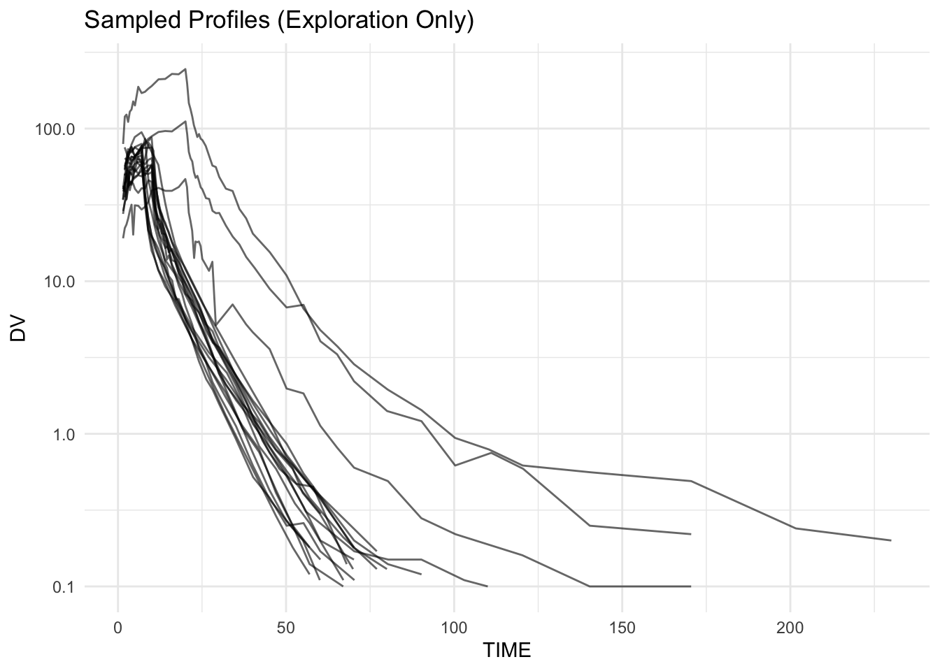
Warning
Sampling can hide extremes.
Never rely on sampled plots for QC conclusions.
Strategy 3: Robust Summaries (Median + IQR)
remi_summary <- remi %>%
  group_by(NOM_TIME) %>%
  summarise(
    median_DV = median(DV),
    q25 = quantile(DV, 0.25),
    q75 = quantile(DV, 0.75),
    n = n(),
    .groups = "drop"
  ) %>%
  arrange(NOM_TIME)

ggplot(remi_summary, aes(NOM_TIME)) +
  geom_ribbon(aes(ymin = q25, ymax = q75), alpha = 0.3) +
  geom_line(aes(y = median_DV), linewidth = 1, linetype = "dashed") +
  scale_y_log10() +
  labs(title = "Median and IQR Summary (Nominal Time)") +
  theme_minimal()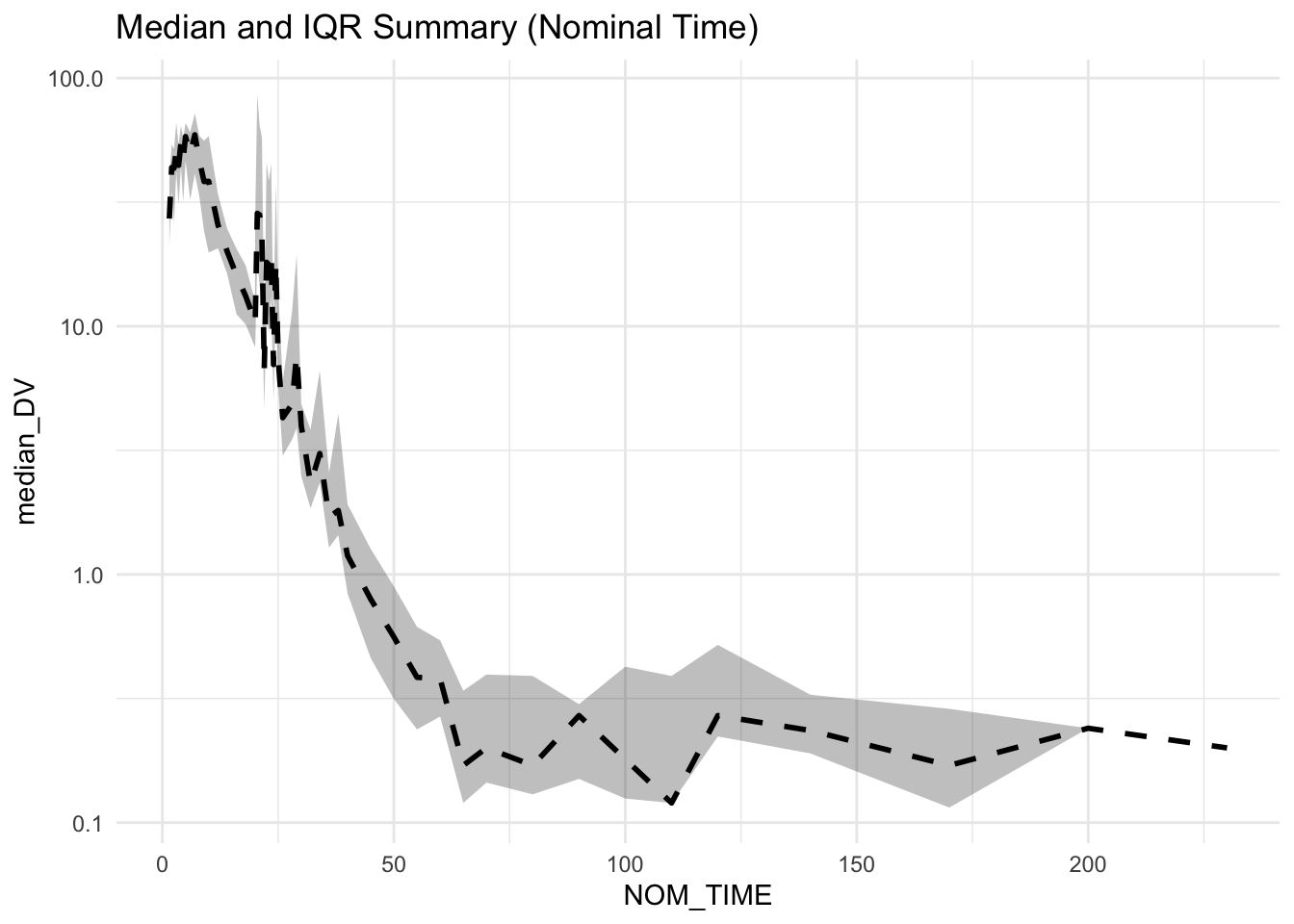
Note
You may notice small “spikes” or wiggles in the summary curve. Remifentanil was administered as an intravenous infusion with varying rates. At certain nominal times, subjects may be in different infusion phases, which can create local structure in population summaries. Not every feature of a summary curve reflects random variability — some reflect study design.
Strategy 4: Balanced View (Individuals + Summary)
ggplot(remi, aes(TIME, DV, group = ID)) +
  geom_line(alpha = 0.05, color = "grey50") +
  geom_ribbon(data = remi_summary,
              aes(NOM_TIME, ymin = q25, ymax = q75),
              inherit.aes = FALSE,
              alpha = 0.3) +
  geom_line(data = remi_summary,
            aes(NOM_TIME, median_DV),
            inherit.aes = FALSE,
            linewidth = 1,
            linetype = "dashed") +
  scale_y_log10() +
  labs(title = "Individuals + Robust Summary (Nominal Time)") +
  theme_minimal()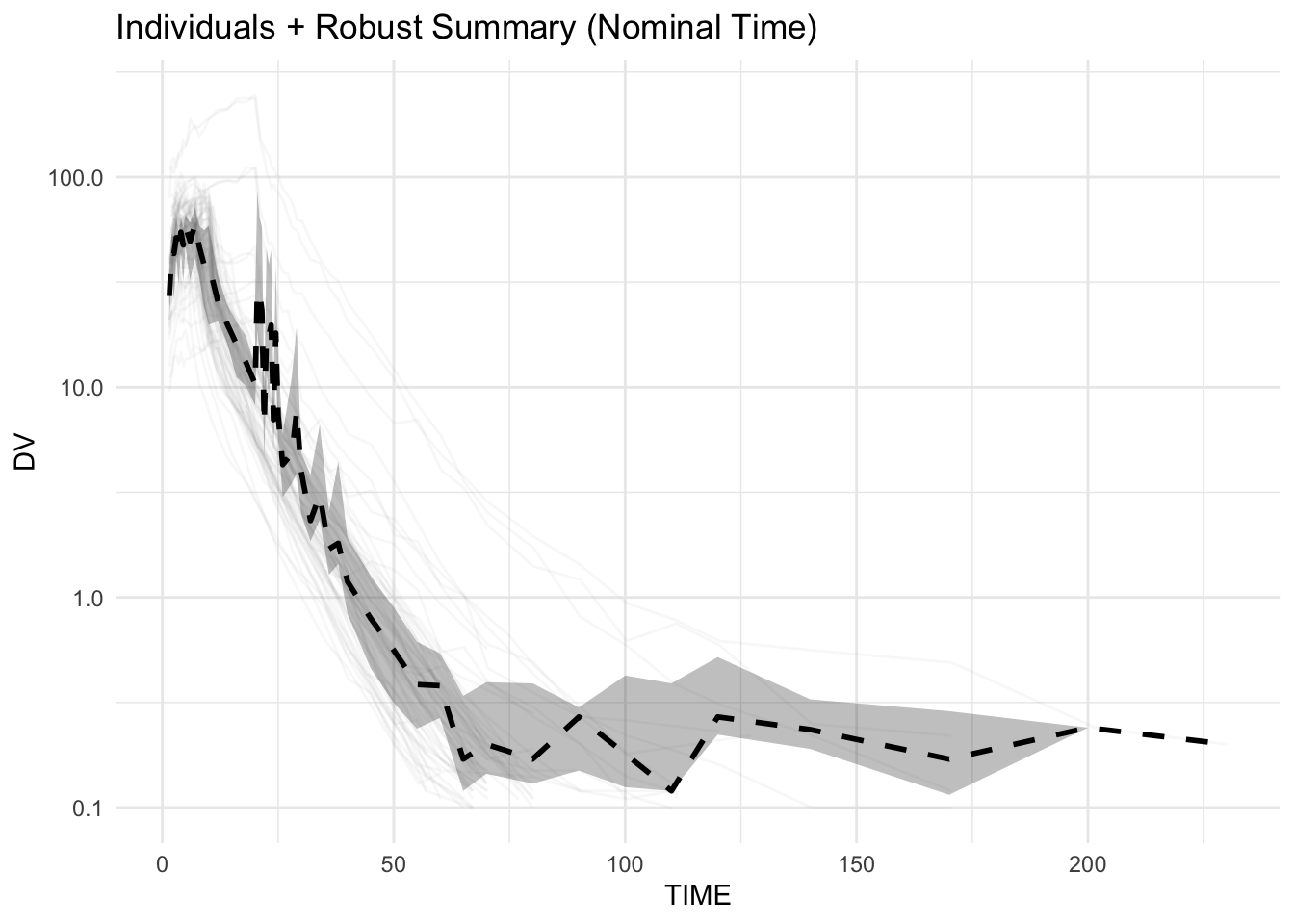
Strategies
- Align time before summarizing.
- Start with alpha blending for large N.
- Use robust summaries (median/IQR).
- Combine individuals and summaries when possible.
- Treat summaries as structure, not truth.
Common Mistakes
- Computing summaries directly on raw time without defining nominal or aligned time.
- Mixing individual and summary layers without clearly distinguishing them visually.
- Using mean ± SD mechanically without considering whether variability is additive or multiplicative.
- Applying multiple compression strategies at once (e.g., sampling + summaries) without understanding their combined effect.
- Treating summary curves as ground truth instead of approximations.
- Not revisiting individual data after seeing an unexpected summary pattern.
- Over-relying on summaries instead of using them alongside individual-level views.
Practice Problems
- Plot individuals only for Remifentanil and identify overplotting.
- Apply alpha blending and compare.
- Align observations to
NOM_TIMEand compute summaries in log space. - Back-transform the log summaries to obtain geometric mean and multiplicative variability bands.
- Compare mean ± SD (additive) to geometric mean ± SD (multiplicative).
Write two sentences explaining why they differ on a log scale.
TipStep-by-Step Solutions
# 1) Individuals only
ggplot(remi, aes(TIME, DV, group = ID)) +
  geom_line(alpha = 0.1) +
  scale_y_log10() +
  theme_minimal()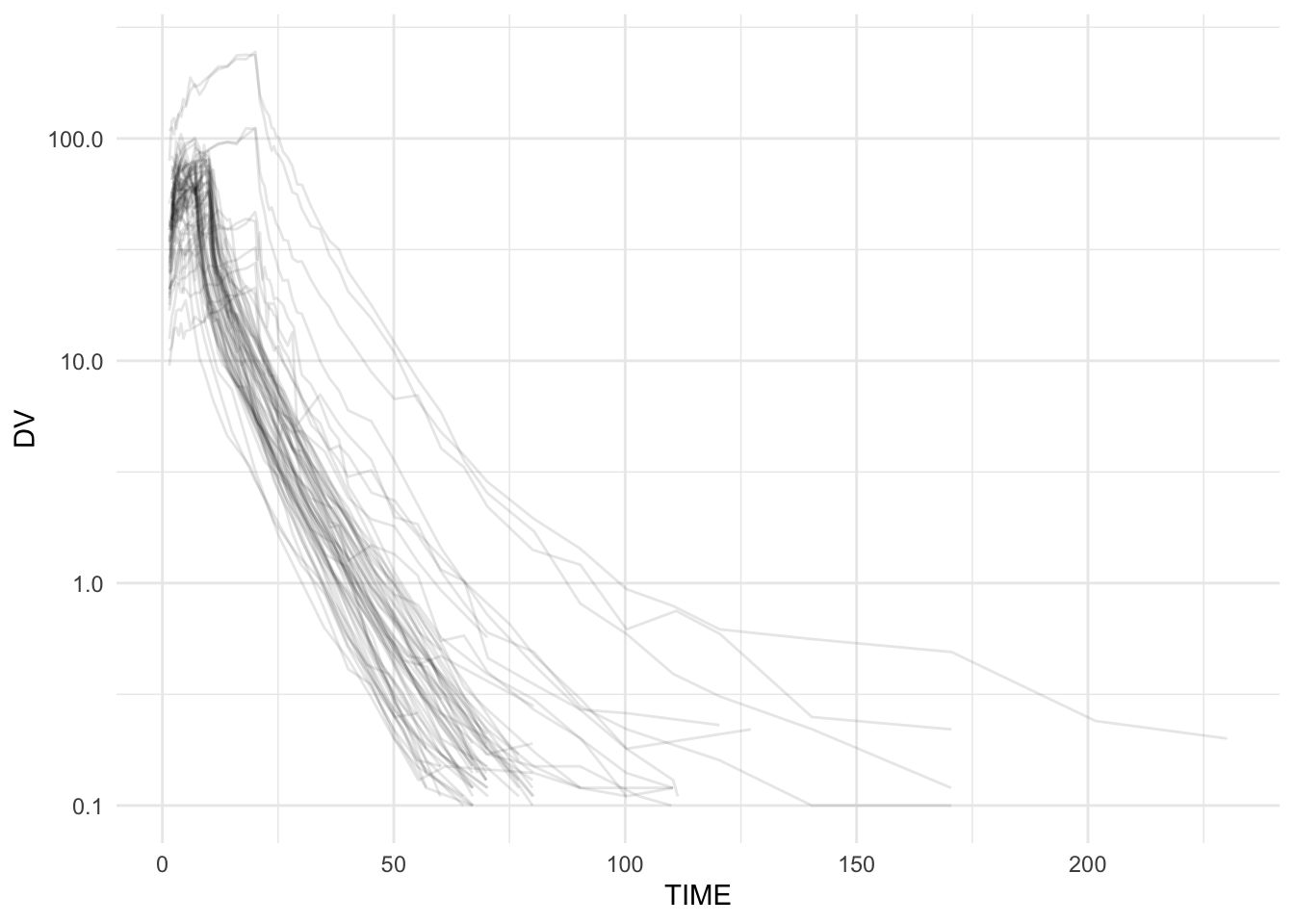
# 2) Alpha blending
ggplot(remi, aes(TIME, DV, group = ID)) +
  geom_line(alpha = 0.05, color = "grey40") +
  scale_y_log10() +
  theme_minimal()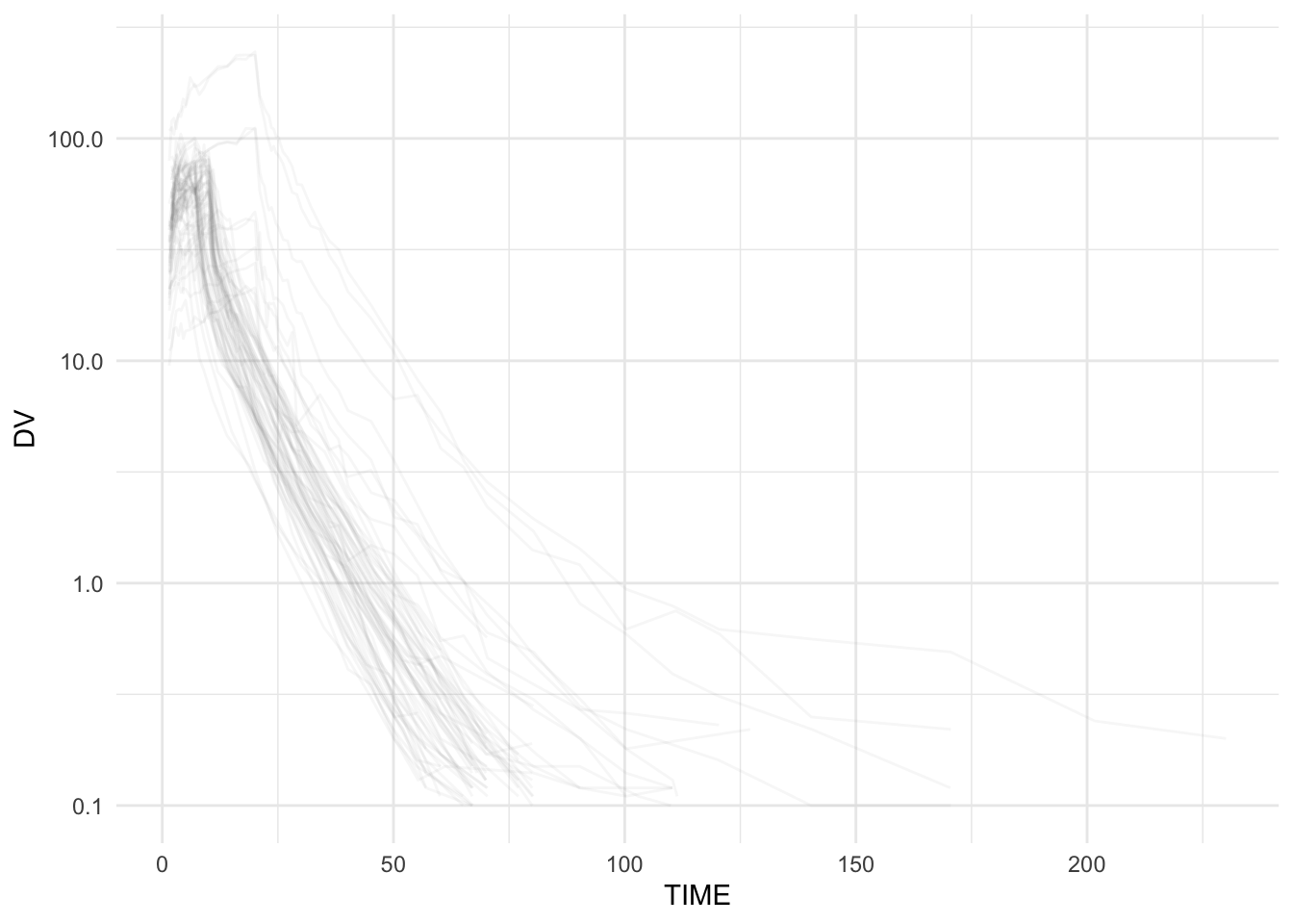
# 3) Log-space summaries by NOM_TIME
remi_log_summary <- remi %>%
  group_by(NOM_TIME) %>%
  summarise(
    n = n(),
    mean_log = mean(log(DV)),
    sd_log   = sd(log(DV)),
    .groups = "drop"
  ) %>%
  filter(n > 1) %>%
  mutate(
    geo_mean = exp(mean_log),
    lower = exp(mean_log - sd_log),
    upper = exp(mean_log + sd_log)
  )

# 4) Plot geometric mean ± SD (multiplicative ribbon)
ggplot(remi_log_summary, aes(NOM_TIME, geo_mean)) +
  geom_ribbon(aes(ymin = lower, ymax = upper), alpha = 0.3) +
  geom_line(linewidth = 1, linetype = "dashed") +
  scale_y_log10() +
  labs(title = "Geometric Mean ± SD (Log-Space Summary)") +
  theme_minimal()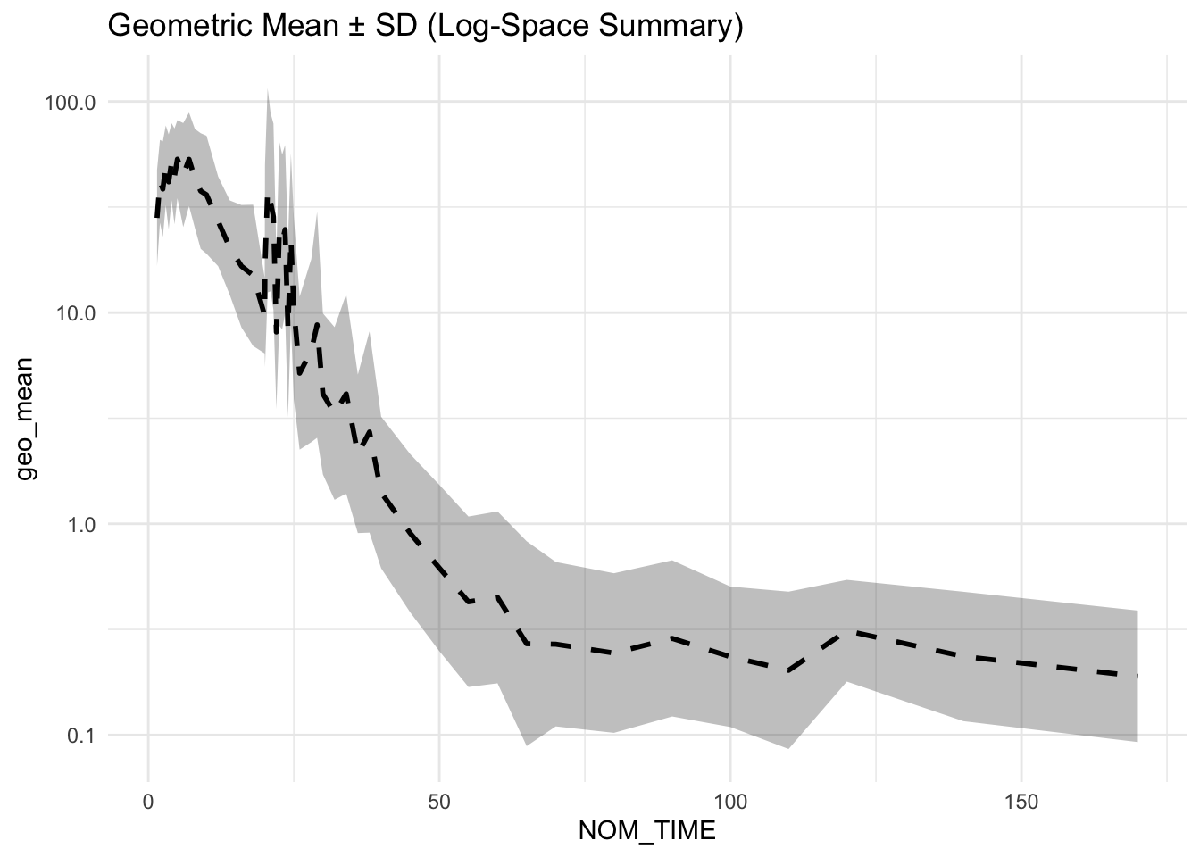
Summary
In this lesson, you learned:
- Summaries require aligned nominal time.
- Mean and SD compress variability.
- Large datasets require visual compression strategies.
- Alpha blending, sampling, binning, and summaries each serve different purposes.
- Responsible visualization balances structure and interpretability.
Visualization is not simplification —
it is controlled compression.
TipQuick Tips
- Summaries are only valid after time alignment (nominal time or bins).
- Start large-N plots with alpha blending before you reach for summaries.
- Prefer median + IQR when outliers or skew are plausible.
- Keep at least one view with individuals visible (even if faint).
- Use
linetypeor a thicker line to make summary layers visually distinct. - If a summary curve surprises you, go back to individuals and investigate.