library(tidyverse)
library(here)
library(nlme)

derivedpath <- here("courses", "foundations-r", "data", "derived")
resultspath <- here("courses", "foundations-r", "results", "modeling", "population")

dir.create(resultspath, recursive = TRUE, showWarnings = FALSE)

final_path <- file.path(derivedpath, "analysis_final_locked.csv")
if (!file.exists(final_path)) {
  stop("Final locked dataset not found. Render the final data assembly lesson first:\n", final_path)
}

analysis <- read_csv(final_path)
obs <- analysis %>% filter(EVID == 0, !is.na(DV), DOSE > 0, is.na(BLQ))Population Modeling with nlme()
Fit a nonlinear mixed-effects one-compartment oral PK model using nlme(), interpret fixed and random effects, perform diagnostics, and formally freeze the model for simulation.
Tip
Big picture: This is the transition from descriptive modeling to decision-capable modeling.
We now estimate a population model, evaluate it carefully, and then freeze it so it can be used for simulation in the next lesson.
Learning Objectives
By the end of this lesson, you will be able to:
- Define a one-compartment oral PK model using log-scale CL/V parameterization.
- Fit a nonlinear mixed-effects model using
nlme(). - Distinguish fixed effects (population means) from random effects (IIV).
- Extract and interpret population and individual parameter estimates.
- Perform core diagnostics (Observed vs Predicted, residuals, ETA checks).
- Extract variance components and compute CV%.
- Save (“freeze”) a fitted model object for downstream simulation.
Key Ideas
- Mixed-effects models combine mechanistic structure with hierarchical variability.
- Fixed effects represent the typical population.
- Random effects represent inter-individual variability (IIV).
- Parameters are modeled on the log scale to enforce positivity.
- After diagnostics are acceptable, the model should be frozen before simulation.
Setup
Worked Example 1: Structural Model (Log-Scale)
We parameterize on the log scale:
\[ k_a = e^{lka}, \quad CL = e^{lCL}, \quad V = e^{lV} \]
one_comp_cl_log <- function(time, dose, lka, lCL, lV) {
  ka <- exp(lka)
  CL <- exp(lCL)
  V  <- exp(lV)
  k  <- CL / V

  (dose * ka / (V * (ka - k))) *
    (exp(-k * time) - exp(-ka * time))
}
This ensures parameters remain positive and improves stability.
Worked Example 2: Fit the Mixed-Effects Model
We allow IIV on CL and V.
nlme_fit <- nlme(
  DV ~ one_comp_cl_log(TIME, DOSE, lka, lCL, lV),
  data = obs,
  fixed  = lka + lCL + lV ~ 1,
  random = lCL + lV ~ 1 | ID,
  start  = c(lka = log(1), lCL = log(5), lV = log(50)),
  control = nlmeControl(maxIter = 200, pnlsTol = 1e-6)
)

summary(nlme_fit)
Nonlinear mixed-effects model fit by maximum likelihood
Model: DV ~ one_comp_cl_log(TIME, DOSE, lka, lCL, lV)
Data: obs
AIC BIC logLik
-302.6961 -277.0311 158.348
Random effects:
Formula: list(lCL ~ 1, lV ~ 1)
Level: ID
Structure: General positive-definite, Log-Cholesky parametrization
StdDev Corr
lCL 0.1387148 lCL
lV 0.2975139 0.293
Residual 0.1240516
Fixed effects: lka + lCL + lV ~ 1
Value Std.Error DF t-value p-value
lka 0.267849 0.07509000 247 3.56705 4e-04
lCL 1.832041 0.05483470 247 33.41025 0e+00
lV 4.213059 0.06502391 247 64.79245 0e+00
Correlation:
lka lCL
lCL -0.386
lV 0.399 -0.151
Standardized Within-Group Residuals:
Min Q1 Med Q3 Max
-7.00496225 -0.35388536 -0.02327382 0.36715655 3.45270883
Number of Observations: 289
Number of Groups: 40 Interpretation:
- Fixed effects → population log-parameters.
- Random effects → subject deviations on the log scale.
Worked Example 3: Population Parameters
fe <- fixef(nlme_fit)

ka_pop <- exp(fe["lka"])
CL_pop <- exp(fe["lCL"])
V_pop  <- exp(fe["lV"])
ke_pop <- CL_pop / V_pop
half_life_pop <- log(2) / ke_pop

pop_params <- tibble(
  ka = ka_pop,
  CL = CL_pop,
  V  = V_pop,
  ke = ke_pop,
  half_life = half_life_pop
)

pop_params
# A tibble: 1 × 5
ka CL V ke half_life
<dbl> <dbl> <dbl> <dbl> <dbl>
1 1.31 6.25 67.6 0.0925 7.50Worked Example 4: Variability (CV%)
vc <- VarCorr(nlme_fit)
omega2_CL <- as.numeric(vc["lCL", "Variance"])
omega2_V  <- as.numeric(vc["lV", "Variance"])

cv_CL <- sqrt(exp(omega2_CL) - 1) * 100
cv_V  <- sqrt(exp(omega2_V) - 1) * 100

tibble(CV_CL_percent = cv_CL,
       CV_V_percent  = cv_V)
# A tibble: 1 × 2
CV_CL_percent CV_V_percent
<dbl> <dbl>
1 13.9 30.4This expresses log-scale variance as interpretable %CV.
Worked Example 5: Individual vs Population Predictions
obs <- obs %>%
  mutate(
    pred_ind = fitted(nlme_fit),
    pred_pop = predict(nlme_fit, level = 0)
  )

p <- ggplot(obs, aes(TIME, DV)) +
  geom_point(alpha = 0.4) +
  geom_line(aes(y = pred_ind, group = ID), alpha = 0.3) +
  geom_line(aes(y = pred_pop), color = "red", linewidth = 1) +
  facet_wrap(~ DOSE) +
  labs(
    title = "Population (red) vs Individual (gray) Predictions",
    x = "Time After Dose (h)",
    y = "Concentration"
  )

p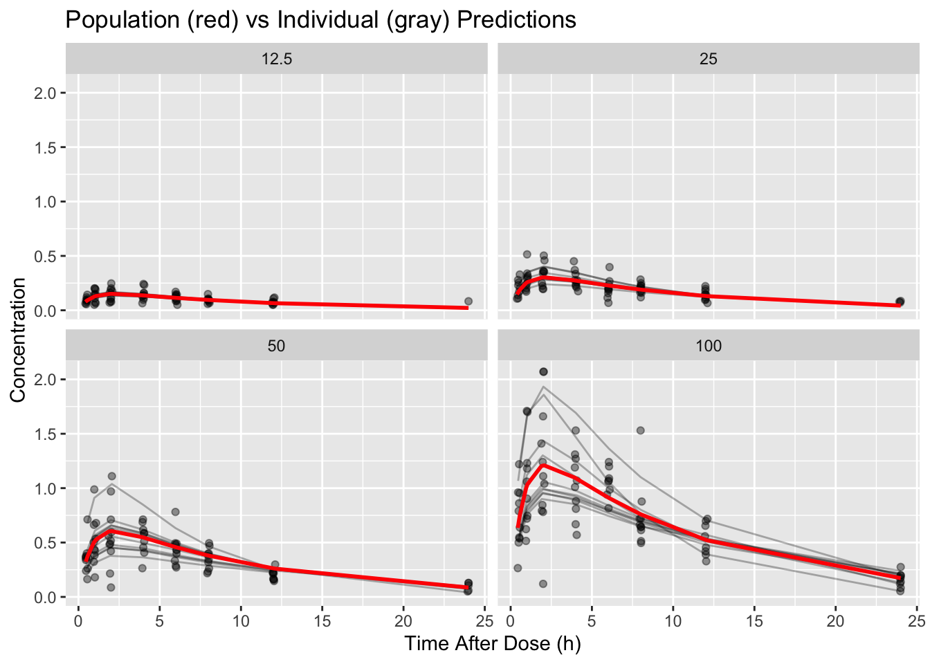
Worked Example 6: Individual View (Faceted by Subject)
Dose facets are great for seeing overall behavior, but they can hide subject-specific fit issues (e.g., one subject consistently above/below).
Now that placebo is excluded, we can facet by all subjects to inspect individual fit quality directly.
obs_pred <- obs %>%
  mutate(
    pred_ind = fitted(nlme_fit),              # conditional (includes random effects)
    pred_pop = predict(nlme_fit, level = 0)   # marginal (fixed effects only)
  )
p_subj <- ggplot(obs_pred, aes(TIME, DV)) +
geom_point(alpha = 0.6) +
geom_line(aes(y = pred_ind, group = ID), alpha = 0.6) +
geom_line(aes(y = pred_pop), color = "red", linewidth = 1) +
facet_wrap(~ ID) +
labs(
title = "nlme Fit: Individual Profiles (All Subjects)",
x = "Time After Dose (h)",
y = "Concentration"
)
p_subj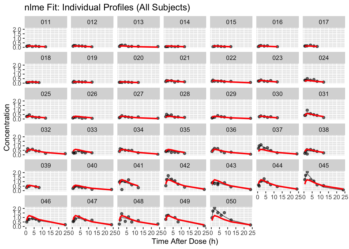
Save:
ggsave(file.path(resultspath, "nlme_fit_all_subjects.png"), p_subj, width = 12, height = 9)Worked Example 7: Residual Diagnostics
obs <- obs %>%
  mutate(resid_pearson = resid(nlme_fit, type = "pearson"))

ggplot(obs, aes(pred_ind, resid_pearson)) +
  geom_point(alpha = 0.4) +
  geom_hline(yintercept = 0, linetype = 2) +
  labs(
    title = "Pearson Residuals vs Fitted",
    x = "Fitted (Individual)",
    y = "Pearson Residual"
  )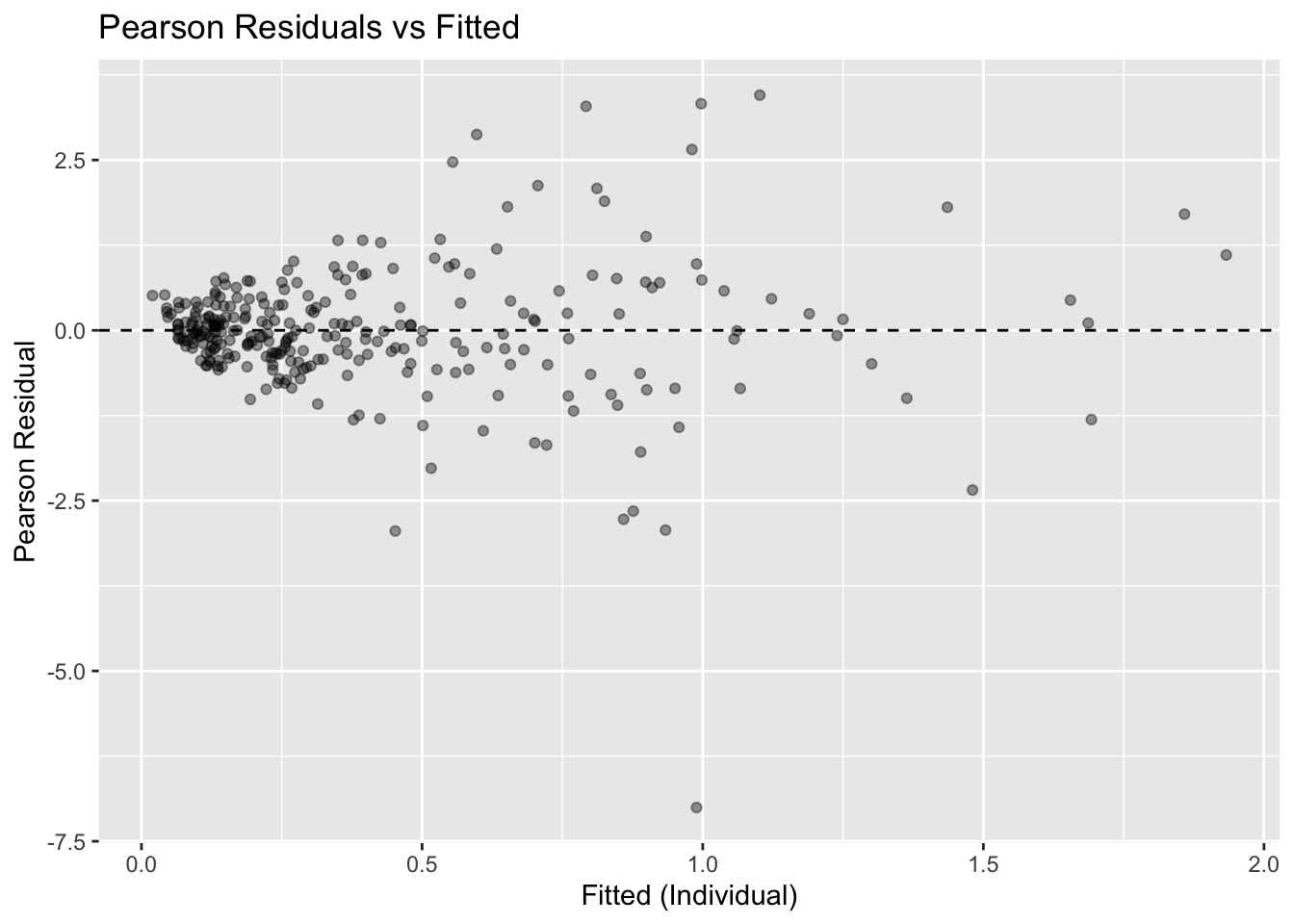
Look for:
- No curvature → structure adequate
- Roughly constant spread → error model plausible
Worked Example 8: Freeze the Model
Once diagnostics are acceptable, freeze the model.
saveRDS(
  nlme_fit,
  file = file.path(resultspath, "nlme_fit.rds")
)
This allows downstream simulation without refitting.
To reload later:
nlme_fit <- readRDS(
  file.path(resultspath, "nlme_fit.rds")
)
Warning
- Do not refit casually once you move to simulation.
- Model freezing preserves reproducibility.
- Always save both parameter tables and the model object.
Strategies
- Start from the locked dataset only.
- Exclude placebo from fitting (
DOSE > 0) because the structural PK model assumes a nonzero administered dose. - Use CL/V parameterization.
- Begin with random effects on CL and V.
- Inspect convergence and variance components.
- Visualize both population and individual predictions.
- Save the model object using
saveRDS().
Common Mistakes
- Treating fixed effects as if they were subject-specific estimates.
- Adding random effects before the simpler model is understood.
- Ignoring convergence messages or variance estimates near zero.
- Comparing population and individual predictions without knowing which level was used.
- Moving to simulation without saving the exact fitted model object.
Practice Problems
- Add random effects on ka. Does stability change?
- Compute shrinkage-like approximation by comparing SD of ETAs to theoretical SD.
- Compare naive pooled CL to population CL.
- Save a CSV summary of fixed effects.
TipStep-by-Step Solutions
Problem 1
nlme(
  DV ~ one_comp_cl_log(TIME, DOSE, lka, lCL, lV),
  data = obs,
  fixed  = lka + lCL + lV ~ 1,
  random = lka + lCL + lV ~ 1 | ID,
  start  = c(lka = log(1), lCL = log(5), lV = log(50))
)
Nonlinear mixed-effects model fit by maximum likelihood
Model: DV ~ one_comp_cl_log(TIME, DOSE, lka, lCL, lV)
Data: obs
Log-likelihood: 163.9971
Fixed: lka + lCL + lV ~ 1
lka lCL lV
0.3184302 1.8296249 4.2134691
Random effects:
Formula: list(lka ~ 1, lCL ~ 1, lV ~ 1)
Level: ID
Structure: General positive-definite, Log-Cholesky parametrization
StdDev Corr
lka 0.4370326 lka lCL
lCL 0.1574259 -0.466
lV 0.3167522 0.401 0.057
Residual 0.1169245
Number of Observations: 289
Number of Groups: 40 Problem 2
eta_sd <- apply(ranef(nlme_fit), 2, sd)
eta_sd
lCL lV
0.06928574 0.24185685 Problem 3
CL_pop lCL
6.246623 Conceptually compare to naive result from prior lesson.
Problem 4
write_csv(
  as.data.frame(fixef(nlme_fit)),
  file.path(resultspath, "fixed_effects_summary.csv")
)
Summary
- You fit a nonlinear mixed-effects PK model.
- You interpreted population and variability parameters.
- You performed core diagnostics.
- You quantified inter-individual variability.
- You froze the model for simulation.
TipQuick Tips
- Model on the log scale.
- Start simple (random CL and V).
- Always visualize predictions.
- Convert variance to %CV for interpretability.
- Freeze the model before simulation.