library(tidyverse)

data(Theoph)

terminal_data <- Theoph %>%
filter(Time >= 4)Variability and Hierarchy: Mixed-Effects Intuition
Pooled vs Separate vs Hierarchical Thinking with Theoph
Learning Objectives
By the end of this lesson, you will be able to:
- Explain why PK data are inherently hierarchical
- Distinguish pooled, separate, and mixed-effects approaches
- Understand random intercepts and random slopes conceptually
- Recognize why repeated-measures data violate independence
- Connect elimination-rate variability to random slopes
Key Ideas
- PK concentration–time data contain repeated measures per subject.
- Pooled models ignore between-subject variability.
- Separate models ignore shared biological structure.
- Mixed-effects models combine population structure with subject variability.
- Random effects represent systematic subject-level deviation — not noise.
Worked Example 1: Visualizing Hierarchy (Theoph)
We return to the Theophylline dataset.
Plot log concentration vs time:
terminal_data %>%
  ggplot(aes(Time, log(conc), group = Subject)) +
  geom_point() +
  geom_line(alpha = 0.6) +
  labs(
    title = "Terminal Phase (Log Scale) — By Subject",
    x = "Time (h)",
    y = "log(Concentration)"
  )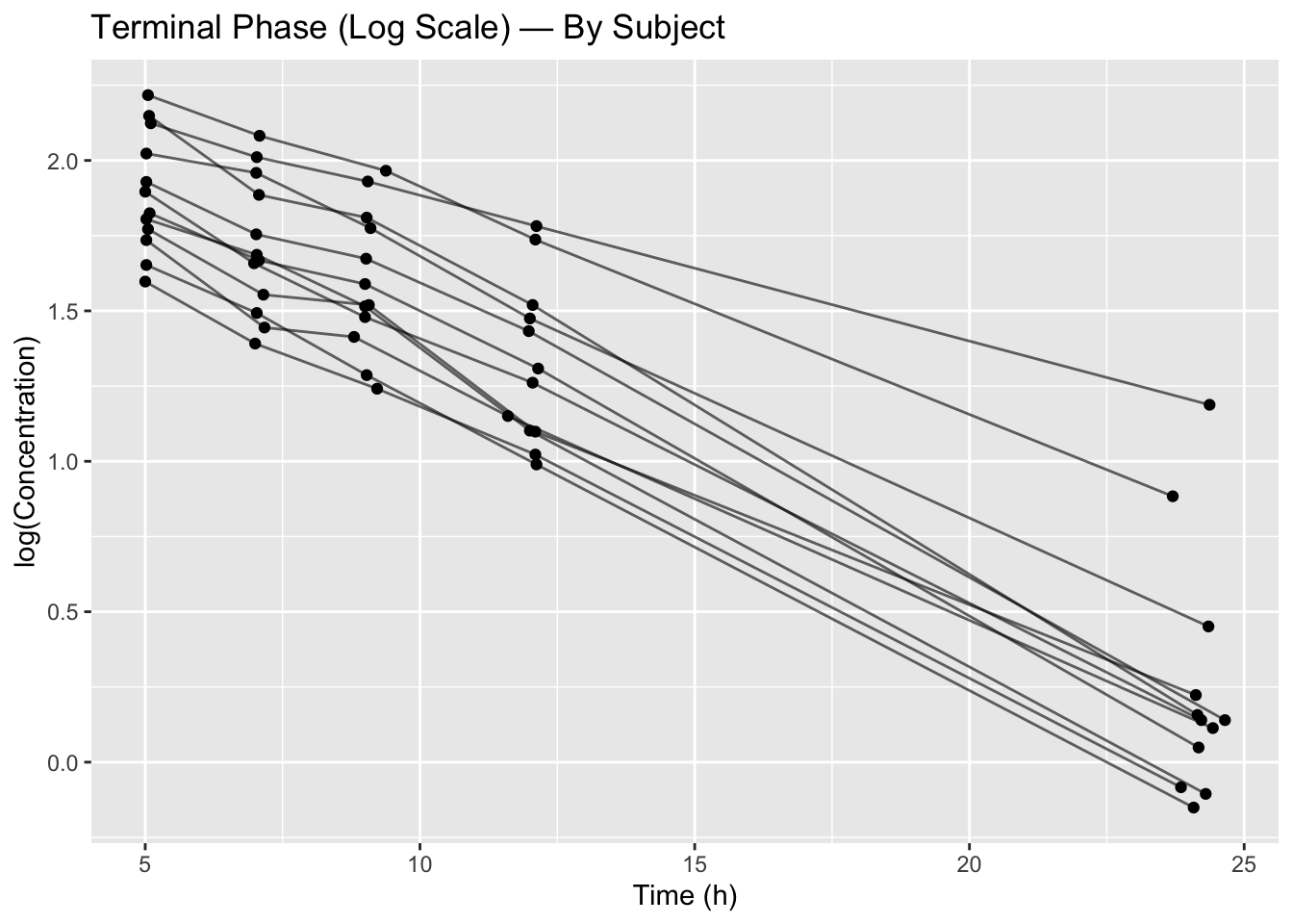
Observe:
- Approximately linear decline per subject
- Different slopes across subjects
- Different intercepts across subjects
This is hierarchy.
Worked Example 2: Pooled Model (Ignoring Hierarchy)
Suppose we fit:
\[ \log(C_{ij}) = \beta_0 + \beta_1 Time_{ij} + \epsilon_{ij} \]
Where:
- \(i\) = subject index
- \(j\) = observation within subject
- \(\beta_0\) = common intercept
- \(\beta_1\) = common slope
- \(\epsilon_{ij}\) = residual error
This assumes:
- One common slope (elimination rate)
- One common intercept
- Independent residuals
Conceptually simple — biologically unrealistic.
Worked Example 3: Separate Models (No Sharing)
Now imagine fitting one linear model per subject:
\[ \log(C_{ij}) = \beta_{0i} + \beta_{1i} Time_{ij} + \epsilon_{ij} \]
This respects subject variability but:
- Uses little data per subject
- Produces unstable estimates
- Provides no population-level summary
Worked Example 4: Hierarchical (Mixed-Effects) Thinking
Mixed-effects modeling assumes:
Population parameters:
\[ \beta_0, \beta_1 \]
Subject-level deviations:
\[ \beta_{0i} = \beta_0 + b_{0i} \]
\[ \beta_{1i} = \beta_1 + b_{1i} \]
Where:
- \(b_{0i}\) = random intercept (baseline variability)
- \(b_{1i}\) = random slope (elimination rate variability)
This preserves shared structure while modeling variability.
Biological Interpretation
In PK terms:
- Random intercept → variability in apparent initial concentration
- Random slope → variability in elimination rate constant (ke)
- Residual error → measurement noise or model misspecification
Variability is not noise — it is biological heterogeneity.
Why Independence Fails
Repeated measures per subject create correlated errors.
If ignored:
- Standard errors are underestimated
- Confidence intervals are too narrow
- Inference becomes unreliable
This is why mixed-effects models are necessary.
Strategies
- Visualize subject-level trajectories.
- Compare pooled vs subject-specific fits conceptually.
- Think in layers: population → subject → observation.
- Translate variability into biological language (e.g., elimination rate differences).
Common Mistakes
- Treating repeated observations as independent
- Assuming variability is just random noise
- Thinking pooled models represent all subjects well
- Fitting each subject separately without considering shared structure
- Confusing residual error with between-subject variability
- Assuming random effects are measurement error
- Ignoring differences in subject-level slopes
- Forgetting that hierarchy exists even before formal mixed-effects modeling
Practice Problems
- In one sentence, explain why pooled modeling underestimates uncertainty.
- Explain why fitting each subject separately wastes information.
- What PK parameter corresponds to a random slope in this context?
- Why is hierarchy the correct data-generating assumption?
TipStep-by-Step Solutions
Problem 1
Because repeated observations within subjects are correlated but treated as independent.
Problem 2
Because each subject’s data are limited, leading to unstable parameter estimates.
Problem 3
The elimination rate constant (ke).
Problem 4
Because PK data arise from population-level biology with subject-level variation and measurement noise.
Summary
- PK data are hierarchical by nature.
- Pooled models ignore variability.
- Separate models ignore shared structure.
- Mixed-effects models combine both ideas.
- This prepares us to fit mixed-effects models formally in the next lesson.
TipQuick Tips
- Always visualize variability first.
- Variability reflects biological differences.
- Random slopes often correspond to elimination differences.
- Mixed-effects modeling is population thinking with structure.