Final Dataset Lock & Exploratory Data Analysis

Lock the cleaned dataset structure, produce disposition summaries, and run disciplined EDA to confirm modeling readiness.

Tip

Big picture: This is the last stop before modeling.
We lock the dataset structure, verify disposition counts, and run focused EDA — not ad hoc exploration.

Learning Objectives

By the end of this lesson, you will be able to:

• Load the cleaned v2 dataset and validate structural integrity.
• Confirm final record counts and subject disposition.
• Build a simple data disposition table (what was kept, dropped, and why).
• Produce covariate summaries suitable for a modeling report.
• Generate dose-stratified concentration profiles (linear + semi-log).
• Summarize BLQ patterns by dose and time.
• Export a locked, modeling-ready dataset and a small set of EDA artifacts.

---

Key Ideas

• Locking means: “this is the dataset we model.” Any change after this must create a new version.
• EDA should answer structured questions:
  • Do profiles look plausible by dose?
  • Are times and counts consistent with protocol?
  • Are covariates in reasonable ranges?
  • Is BLQ behavior consistent with time/dose?
• Save what you use to decide: tables + plots are part of the deliverable.

---

Setup

library(tidyverse)
library(here)

derivedpath <- here("courses", "foundations-r", "data", "derived")
resultspath <- here("courses", "foundations-r", "results", "eda")
qcpath      <- here("courses", "foundations-r", "results", "qc")

dir.create(resultspath, recursive = TRUE, showWarnings = FALSE)

clean_path <- file.path(derivedpath, "analysis_v2_cleaned.csv")
if (!file.exists(clean_path)) {
  stop("Cleaned dataset not found. Render the previous lesson first:\n", clean_path)
}

analysis <- read_csv(clean_path)

obs  <- analysis %>% filter(EVID == 0)
dose <- analysis %>% filter(EVID == 1)

---

Worked Example 1: Final Disposition Counts

Start with the simplest checks: subjects, rows, obs, doses.

tibble(
  n_subjects = n_distinct(analysis$ID),
  n_total_rows = nrow(analysis),
  n_obs = nrow(obs),
  n_dose = nrow(dose)
)

# A tibble: 1 × 4
  n_subjects n_total_rows n_obs n_dose
       <int>        <int> <int>  <int>
1         50          492   442     50

Record counts per subject:

analysis %>%
  count(ID) %>%
  count(n) %>%
  arrange(n)

# A tibble: 3 × 2
      n    nn
  <int> <int>
1     8     3
2     9     2
3    10    45

Dose row validation (must be exactly 1 dose row per subject):

dose_check <- analysis %>%
  filter(EVID == 1) %>%
  count(ID) %>%
  filter(n != 1)

dose_check

# A tibble: 0 × 2
# ℹ 2 variables: ID <chr>, n <int>

Save any problematic IDs (if present):

write_csv(dose_check, file.path(resultspath, "dose_row_validation.csv"))

---

Worked Example 2: Data Disposition Table

Even though we are now working from the cleaned dataset, we can still summarize what changed using the evidence files created in the previous lesson.

If you ran the previous lesson, you should have evidence CSVs under results/qc/. We’ll build a lightweight disposition table from what exists.

evidence_files <- c(
  "evidence_missing_time_obs.csv",
  "evidence_duplicate_rows.csv",
  "evidence_negative_dv.csv",
  "evidence_wt_unit_suspects.csv"
)

evidence_paths <- file.path(qcpath, evidence_files)

disposition <- tibble(
  issue = c(
    "Missing TIME (obs rows dropped)",
    "Exact duplicates removed (ID + TIME)",
    "Negative DV handled (set to NA)",
    "WT unit mismatch fixed (lb→kg)"
  ),
  evidence_file = evidence_files,
  available = file.exists(evidence_paths)
)

disposition

# A tibble: 4 × 3
  issue                                evidence_file                 available
  <chr>                                <chr>                         <lgl>    
1 Missing TIME (obs rows dropped)      evidence_missing_time_obs.csv TRUE     
2 Exact duplicates removed (ID + TIME) evidence_duplicate_rows.csv   TRUE     
3 Negative DV handled (set to NA)      evidence_negative_dv.csv      TRUE     
4 WT unit mismatch fixed (lb→kg)       evidence_wt_unit_suspects.csv TRUE     

Add counts where possible:

get_nrows_if_exists <- function(p) if (file.exists(p)) nrow(read_csv(p, show_col_types = FALSE)) else NA_integer_

disposition <- disposition %>%
  mutate(
    n_rows_flagged = purrr::map_int(evidence_paths, get_nrows_if_exists)
  )

write_csv(disposition, file.path(resultspath, "data_disposition_summary.csv"))
disposition

# A tibble: 4 × 4
  issue                                evidence_file    available n_rows_flagged
  <chr>                                <chr>            <lgl>              <int>
1 Missing TIME (obs rows dropped)      evidence_missin… TRUE                   8
2 Exact duplicates removed (ID + TIME) evidence_duplic… TRUE                  16
3 Negative DV handled (set to NA)      evidence_negati… TRUE                   1
4 WT unit mismatch fixed (lb→kg)       evidence_wt_uni… TRUE                   0

---

Worked Example 3: Covariate Summaries (Subject-Level)

Create a one-row-per-subject covariate table.

subj <- analysis %>%
  distinct(ID, DOSE, AGE, WT, SEX)

subj %>% slice_head(n = 10)

# A tibble: 10 × 5
   ID     DOSE   AGE    WT SEX  
   <chr> <dbl> <dbl> <dbl> <chr>
 1 001       0    42  70.6 M    
 2 002       0    34  75.5 male 
 3 003       0    45  67.2 M    
 4 004       0    37 111   male 
 5 005       0    59  83.8 M    
 6 006       0    43  60.7 F    
 7 007       0    52  94.1 F    
 8 008       0    52  73.9 F    
 9 009       0    59  97.5 F    
10 010       0    60  68.8 F    

Overall summaries:

cov_summary <- subj %>%
  pivot_longer(
    cols = c(AGE, WT),
    names_to = "covariate",
    values_to = "value"
  ) %>%
  group_by(covariate) %>%
  summarise(
    n_subjects = sum(!is.na(value)),
    min = min(value, na.rm = TRUE),
    median = median(value, na.rm = TRUE),
    max = max(value, na.rm = TRUE),
    .groups = "drop"
  )

cov_summary

# A tibble: 2 × 5
  covariate n_subjects   min median   max
  <chr>          <int> <dbl>  <dbl> <dbl>
1 AGE               48  30     44.5    60
2 WT                48  44.4   73.2   113

Using pivot_longer() creates a scalable workflow where all covariates are handled in a single consistent structure. Instead of writing separate summary code for each variable (AGE, WT, etc.), we can summarize any number of covariates using the same grouped workflow.

By sex:

cov_by_sex <- subj %>%
  group_by(SEX) %>%
  summarise(
    n = n(),
    age_median = median(AGE, na.rm = TRUE),
    wt_median = median(WT, na.rm = TRUE),
    .groups = "drop"
  )

cov_by_sex

# A tibble: 4 × 4
  SEX        n age_median wt_median
  <chr>  <int>      <dbl>     <dbl>
1 F         23       43.5      69.8
2 Female     3       39        71.4
3 M         21       49        74.8
4 male       3       37        75.5

Save:

write_csv(cov_summary, file.path(resultspath, "covariate_summary_overall.csv"))
write_csv(cov_by_sex, file.path(resultspath, "covariate_summary_by_sex.csv"))

Optional: quickly scan for “still suspicious” WT values:

subj %>% filter(!is.na(WT) & WT > 150) %>% arrange(desc(WT))

# A tibble: 0 × 5
# ℹ 5 variables: ID <chr>, DOSE <dbl>, AGE <dbl>, WT <dbl>, SEX <chr>

---

Worked Example 4: Profiles by DOSE (Semi-Log)

p_log <- ggplot(obs, aes(x = TIME, y = DV, group = ID)) +
  geom_line(alpha = 0.3) +
  geom_point(size = 0.8) +
  facet_wrap(~DOSE) +
  scale_y_log10() +
  labs(
    title = "Final (v2) Dataset: Concentration–Time Profiles by DOSE (Log Scale)",
    x = "Time After Dose (h)",
    y = "Concentration"
  )

p_log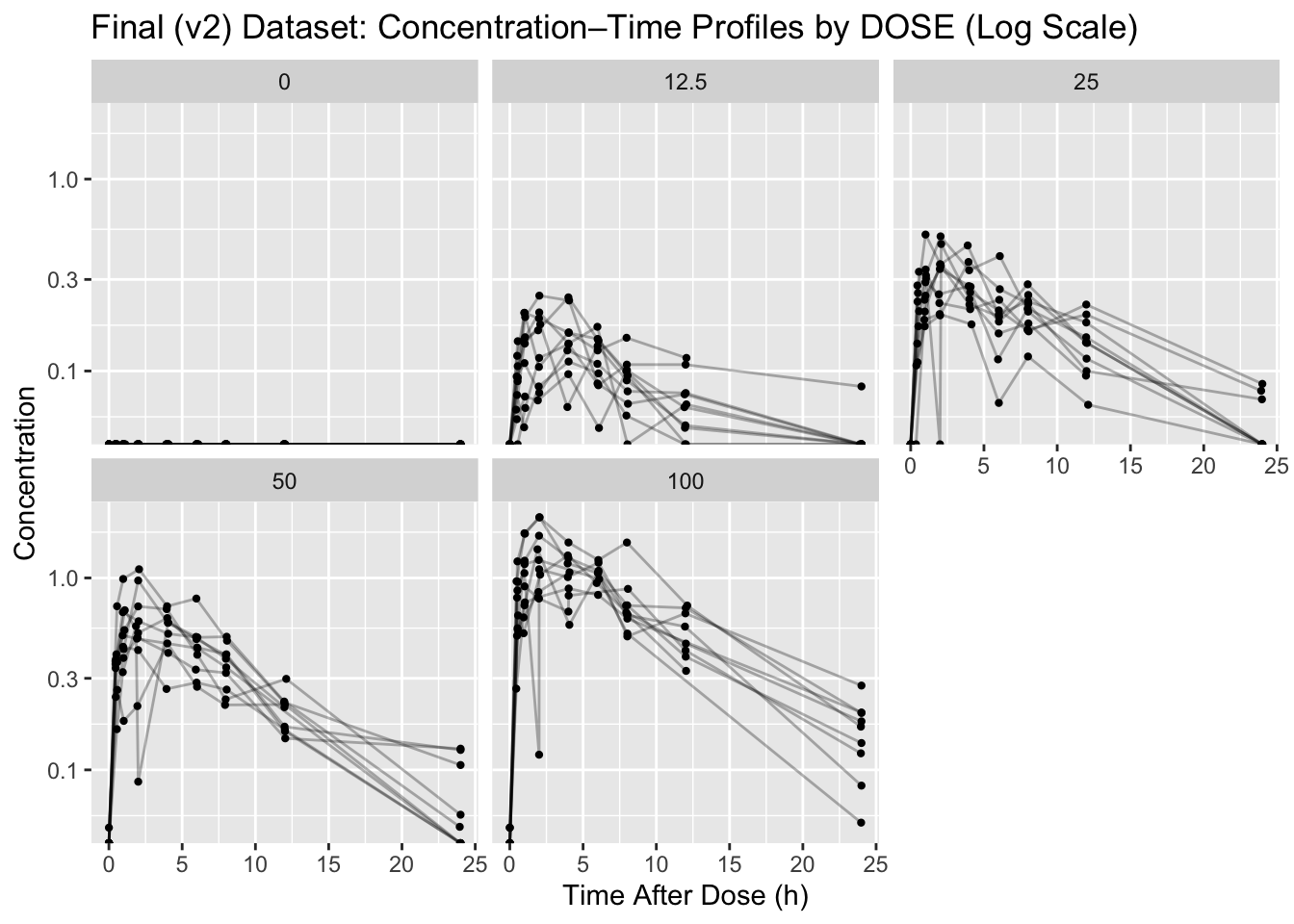

Save:

ggsave(file.path(resultspath, "profiles_by_dose_log.png"), p_log, width = 9, height = 6)

---

Worked Example 5: Profiles by DOSE (Linear)

Linear scale is useful to see spikes near Cmax and understand absolute differences.

p_lin <- ggplot(obs, aes(x = TIME, y = DV, group = ID)) +
  geom_line(alpha = 0.3) +
  geom_point(size = 0.8) +
  facet_wrap(~DOSE) +
  labs(
    title = "Final (v2) Dataset: Concentration–Time Profiles by DOSE (Linear Scale)",
    x = "Time After Dose (h)",
    y = "Concentration"
  )

p_lin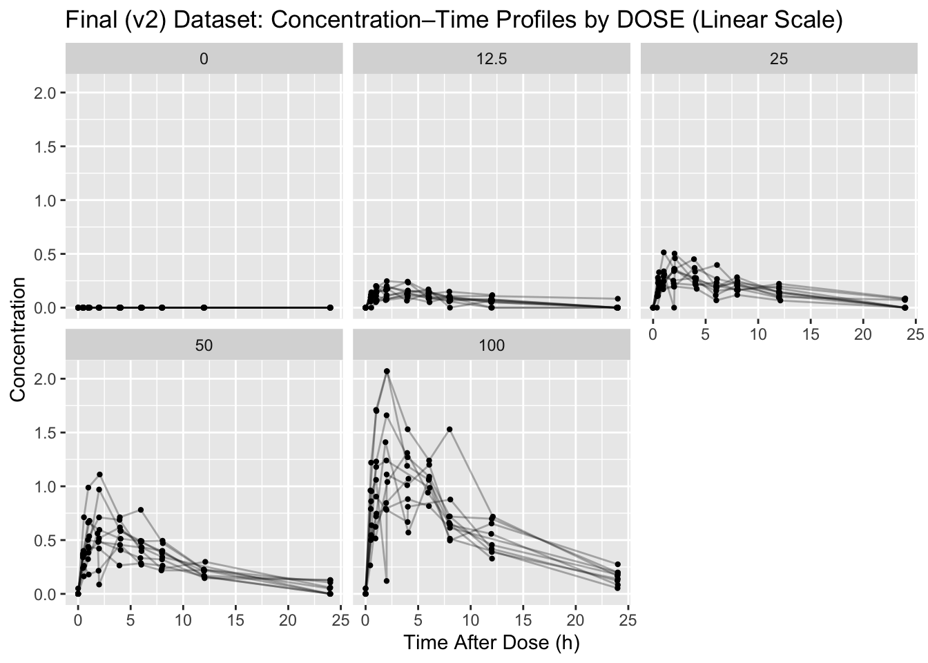

Save:

ggsave(file.path(resultspath, "profiles_by_dose_linear.png"), p_lin, width = 9, height = 6)

---

Worked Example 6: BLQ Summary

BLQ summaries help us understand where concentrations fall below the assay limit of quantification. Patterns in BLQ observations often reveal elimination behavior, sparse late sampling, or potential assay limitations.

BLQ by dose:

blq_by_dose <- obs %>%
  group_by(DOSE) %>%
  summarise(
    n_obs = n(),
    n_blq = sum(BLQ == "BLQ", na.rm = TRUE),
    pct_blq = 100 * n_blq / n_obs,
    .groups = "drop"
  )

blq_by_dose

# A tibble: 5 × 4
   DOSE n_obs n_blq pct_blq
  <dbl> <int> <int>   <dbl>
1   0      88    88   100  
2  12.5    89    22    24.7
3  25      90    18    20  
4  50      88    14    15.9
5 100      87    10    11.5

Placebo or zero-dose groups will naturally contain BLQ observations because no drug exposure is expected. This is scientifically different from unexpectedly high BLQ rates in treated groups.

To focus specifically on BLQ timing patterns in treated subjects, we filter to BLQ rows and exclude DOSE == 0.

blq_by_ntime <- obs %>%
  filter(DOSE > 0, BLQ == "BLQ") %>%
  group_by(DOSE, NTIME) %>%
  summarise(
    n_blq = n(),
    .groups = "drop"
  ) %>%
  arrange(DOSE, NTIME)

blq_by_ntime %>% slice_head(n = 15)

# A tibble: 12 × 3
    DOSE NTIME n_blq
   <dbl> <dbl> <int>
 1  12.5   0      10
 2  12.5   0.5     1
 3  12.5   8       1
 4  12.5  12       2
 5  12.5  24       8
 6  25     0      10
 7  25     0.5     1
 8  25     2       1
 9  25    24       6
10  50     0      10
11  50    24       4
12 100     0      10

All zero-dose records are expected to be BLQ because no drug exposure occurred. In treated subjects, BLQ observations are often expected to increase at later nominal times as concentrations decline during elimination.

Save:

write_csv(blq_by_dose, file.path(resultspath, "blq_summary_by_dose.csv"))
write_csv(blq_by_ntime, file.path(resultspath, "blq_summary_by_dose_ntime.csv"))

---

Worked Example 7: Cmax/Tmax Table (Helpful for Modeling Readiness)

This is a quick “sanity lens” before fitting individual models.

cmax_tbl <- obs %>%
  group_by(ID, DOSE) %>%
  summarise(
    cmax = max(DV, na.rm = TRUE),
    tmax = TIME[which.max(DV)],
    .groups = "drop"
  ) %>%
  arrange(desc(cmax))

cmax_tbl %>% slice_head(n = 10)

# A tibble: 10 × 4
   ID     DOSE  cmax  tmax
   <chr> <dbl> <dbl> <dbl>
 1 045     100  2.07  2.04
 2 050     100  2.07  2.01
 3 042     100  1.66  2.00
 4 048     100  1.41  1.89
 5 044     100  1.31  3.96
 6 049     100  1.24  1.97
 7 041     100  1.2   6.06
 8 037      50  1.11  2.06
 9 047     100  1.07  4.08
10 031      50  0.97  2.00

Save:

write_csv(cmax_tbl, file.path(resultspath, "cmax_tmax_by_subject.csv"))

---

Lock the Dataset

Locking means we write a final, modeling-ready file and treat it as read-only.

final_path <- file.path(derivedpath, "analysis_final_locked.csv")
write_csv(analysis, final_path)

final_path

[1] "/Users/aelmokadem/git/aeacademy-pmx/courses/foundations-r/data/derived/analysis_final_locked.csv"

---

Warning

• Do not modify this dataset after locking.
• Any further changes require a version increment (v3, etc.).
• Modeling lessons should use only analysis_final_locked.csv.
• Save tables/plots used for decisions under results/eda/.

---

Strategies

• Work only from analysis_v2_cleaned.csv.
• Split observation vs dose rows (EVID == 0 vs EVID == 1) for clear checks.
• Build a minimal EDA bundle:
  • disposition table
  • covariate summary table
  • profiles (linear + log)
  • BLQ summary
  • Cmax/Tmax table (optional but useful)
• Save:
  • plots under courses/foundations-r/results/eda/
  • summary tables under courses/foundations-r/results/eda/
  • final locked dataset under courses/foundations-r/data/derived/

---

Common Mistakes

• Treating the v2 dataset as locked before checking dose rows, counts, and keys.
• Running open-ended EDA without saving the tables and plots that supported decisions.
• Mixing observation and dose rows in summaries where they should be separate.
• Ignoring remaining covariate outliers after the unit correction step.
• Continuing to edit the locked dataset without creating a new version.

---

Practice Problems

1. Confirm there are no remaining duplicate observation keys (ID + TIME).
2. Verify there are no remaining negative DV values.
3. Create a subject-level covariate table and save it as results/eda/subject_covariates.csv.
4. Compute median Cmax by DOSE and save it as results/eda/median_cmax_by_dose.csv.

---

TipStep-by-Step Solutions

Duplicate check (obs only):

obs %>%
  count(ID, TIME) %>%
  filter(n > 1)

# A tibble: 0 × 3
# ℹ 3 variables: ID <chr>, TIME <dbl>, n <int>

Negative DV check:

obs %>% filter(!is.na(DV) & DV < 0)

# A tibble: 0 × 13
# ℹ 13 variables: ID <chr>, DOSE <dbl>, TIME <dbl>, NTIME <dbl>, EVID <dbl>,
#   CMT <dbl>, AMT <dbl>, DV <dbl>, AGE <dbl>, WT <dbl>, SEX <chr>, BLQ <chr>,
#   LLOQ <dbl>

Subject covariate table:

subj_cov <- analysis %>%
  distinct(ID, DOSE, AGE, WT, SEX)

write_csv(subj_cov, file.path(resultspath, "subject_covariates.csv"))
subj_cov %>% slice_head(n = 10)

# A tibble: 10 × 5
   ID     DOSE   AGE    WT SEX  
   <chr> <dbl> <dbl> <dbl> <chr>
 1 001       0    42  70.6 M    
 2 002       0    34  75.5 male 
 3 003       0    45  67.2 M    
 4 004       0    37 111   male 
 5 005       0    59  83.8 M    
 6 006       0    43  60.7 F    
 7 007       0    52  94.1 F    
 8 008       0    52  73.9 F    
 9 009       0    59  97.5 F    
10 010       0    60  68.8 F    

Median Cmax by dose:

median_cmax <- obs %>%
  group_by(ID, DOSE) %>%
  summarise(cmax = max(DV, na.rm = TRUE), .groups = "drop") %>%
  group_by(DOSE) %>%
  summarise(median_cmax = median(cmax, na.rm = TRUE), .groups = "drop") %>%
  arrange(DOSE)

write_csv(median_cmax, file.path(resultspath, "median_cmax_by_dose.csv"))
median_cmax

# A tibble: 5 × 2
   DOSE median_cmax
  <dbl>       <dbl>
1   0         0    
2  12.5       0.188
3  25         0.356
4  50         0.624
5 100         1.27 

---

Summary

• You validated that the cleaned dataset is structurally consistent (dose rows, counts, keys).
• You produced a lightweight data disposition summary referencing QC evidence files.
• You summarized covariates and checked for remaining outliers.
• You generated dose-stratified profiles (log + linear) and saved the figures.
• You summarized BLQ patterns and saved tables for reporting.
• You locked the final dataset for modeling as analysis_final_locked.csv.

---

TipQuick Tips

• Locking is a commitment: any change requires a new version.
• Keep EDA questions structured (counts, ranges, shape checks).
• Save artifacts you used to decide (tables + figures).
• Before modeling: confirm one dose row per subject and no duplicate observation keys.