Naive Pooled Modeling with nls()

Fit a one-compartment oral PK model using naive pooled data, interpret structural parameters, and understand the limitations of ignoring inter-individual variability.

Tip

Big picture: Before hierarchical modeling, a common first step is a naive pooled fit.
Here, we ignore inter-individual variability and fit one structural model to all subjects simultaneously.

Learning Objectives

By the end of this lesson, you will be able to:

Define a one-compartment oral PK model using CL/V parameterization.
Perform a naive pooled nonlinear fit using nls().
Interpret ka, CL, V, ke, and half-life from a pooled model.
Generate pooled fitted curves and diagnostics.
Explain the limitations of naive pooled modeling.

Key Ideas

Naive pooling treats all subjects as if they share identical parameters.
Dose differences still affect predictions through the structural equation.
Placebo (DOSE = 0) is excluded from fitting because the model describes post-dose PK after an administered dose.
Between-subject variability is absorbed into residual error.
Parameter estimates represent an “average structural subject.”
This approach is simple but statistically limited.

Setup

library(tidyverse)
library(here)

derivedpath <- here("courses", "foundations-r", "data", "derived")
resultspath <- here("courses", "foundations-r", "results", "modeling", "naive_pooled")

dir.create(resultspath, recursive = TRUE, showWarnings = FALSE)

final_path <- file.path(derivedpath, "analysis_final_locked.csv")
if (!file.exists(final_path)) {
  stop("Final locked dataset not found. Render the final dataset assembly lesson  first:\n", final_path)
}

analysis <- read_csv(final_path)

obs <- analysis %>% filter(EVID == 0, !is.na(DV), DOSE > 0, is.na(BLQ))

Worked Example 1: Structural Model (CL/V Parameterization)

First, we define the concentration-time function that nls() will use during estimation.

\[ C(t) = \frac{D \cdot k_a}{V (k_a - k)} \left(e^{-k t} - e^{-k_a t}\right), \quad k = \frac{CL}{V}. \]

one_comp_cl <- function(time, dose, ka, CL, V) {
  k <- CL / V
  (dose * ka / (V * (ka - k))) *
    (exp(-k * time) - exp(-ka * time))
}

Worked Example 2: Fit Naive Pooled Model

Now we fit one shared set of structural parameters to all non-placebo observations.

naive_fit <- nls(
  DV ~ one_comp_cl(TIME, DOSE, ka, CL, V),
  data = obs,
  start = list(ka = 1, CL = 5, V = 50),
  control = nls.control(maxiter = 200, warnOnly = TRUE)
)

summary(naive_fit)


Formula: DV ~ one_comp_cl(TIME, DOSE, ka, CL, V)

Parameters:
   Estimate Std. Error t value Pr(>|t|)    
ka   1.3787     0.1649   8.361 2.75e-15 ***
CL   6.2273     0.4359  14.287  < 2e-16 ***
V   68.3905     3.4250  19.968  < 2e-16 ***
---
Signif. codes:  0 '***' 0.001 '**' 0.01 '*' 0.05 '.' 0.1 ' ' 1

Residual standard error: 0.1905 on 286 degrees of freedom

Number of iterations to convergence: 5 
Achieved convergence tolerance: 8.536e-07

Interpretation:

One ka, CL, V shared across all subjects.
Differences in profiles arise only from DOSE and residual error.

Worked Example 3: Convert to Interpretable Parameters

The fitted coefficients are useful, but derived quantities such as elimination rate and half-life are easier to interpret.

est <- coef(naive_fit)

ka_pop <- est["ka"]
CL_pop <- est["CL"]
V_pop  <- est["V"]
ke_pop <- CL_pop / V_pop
half_life <- log(2) / ke_pop

tibble(
  ka = ka_pop,
  CL = CL_pop,
  V  = V_pop,
  ke = ke_pop,
  half_life = half_life
)

# A tibble: 1 × 5
     ka    CL     V     ke half_life
  <dbl> <dbl> <dbl>  <dbl>     <dbl>
1  1.38  6.23  68.4 0.0911      7.61

Worked Example 4: Visual Diagnostics

Predictions by subject show where the pooled model follows the general trend and where it misses individual behavior.

Generate predictions:

obs <- obs %>%
  mutate(pred = predict(naive_fit))

Plot by subject:

p <- ggplot(obs, aes(TIME, DV)) +
  geom_point(alpha = 0.6) +
  geom_line(aes(y = pred, group = ID), color = "blue") +
  facet_wrap(~ ID) +
  labs(
    title = "Naive Pooled Fit by Subject",
    x = "Time After Dose (h)",
    y = "Concentration"
  )

p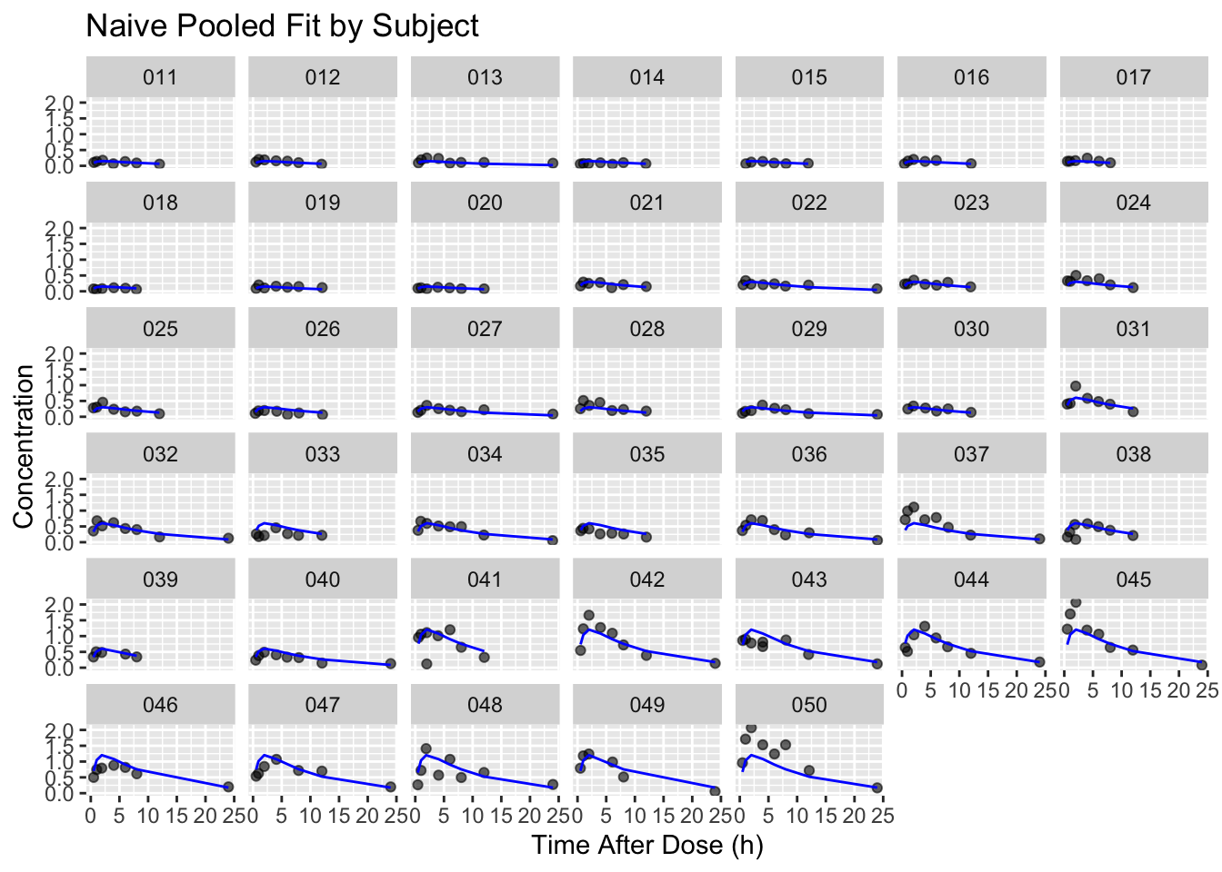

Save:

ggsave(file.path(resultspath, "naive_pooled_fits.png"), p, width = 10, height = 8)

Worked Example 6: Residual Diagnostics

Residual plots help separate random scatter from systematic patterns that suggest model limitations.

obs <- obs %>%
  mutate(residual = DV - pred)

ggplot(obs, aes(pred, residual)) +
  geom_point(alpha = 0.6) +
  geom_hline(yintercept = 0, linetype = 2) +
  labs(
    title = "Residuals vs Fitted (Naive Pooled)",
    x = "Fitted",
    y = "Residual"
  )

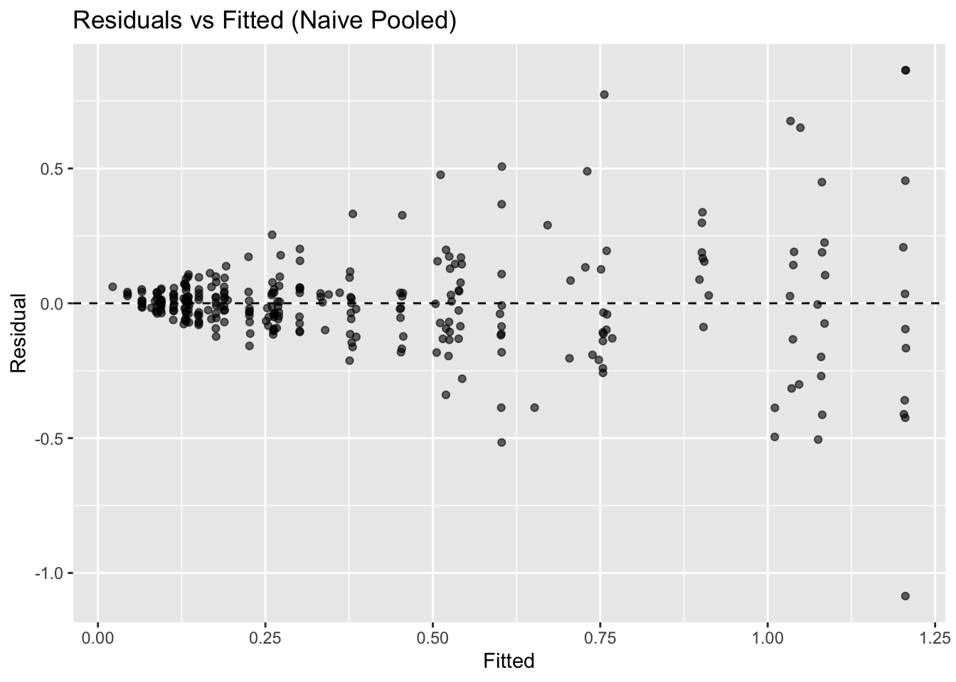
What to look for:

Systematic curvature → structural misspecification.
Increasing spread → heteroscedasticity.
Clustering by subject → ignored inter-individual variability.

In this fit, the residual spread increases at higher fitted concentrations, suggesting heteroscedasticity where variability grows with concentration magnitude. In practice, this often motivates log-transformed modeling or proportional error structures, which are handled more naturally in mixed-effects frameworks such as nlme and nlmixr2.

Warning

Naive pooled models underestimate true variability.
Residual error absorbs between-subject differences.
Do not interpret this as a population PK model.

Strategies

Work from the locked dataset (analysis_final_locked.csv).
Filter to observation rows (EVID == 0).
Use reasonable starting values.
Inspect residual patterns carefully.
Treat results as exploratory, not definitive.

Common Mistakes

Including placebo rows in a model that assumes a nonzero administered dose.
Interpreting naive pooled estimates as population mixed-effects estimates.
Trusting convergence without checking fitted curves and residuals.
Treating between-subject differences as residual noise only.
Using the pooled model for decisions without acknowledging its limitations.

Practice Problems

Stratify residuals by DOSE — do higher doses show larger error?
Create a log-scale concentration plot.
Compute RMSE of the pooled fit.

Step-by-Step Solutions

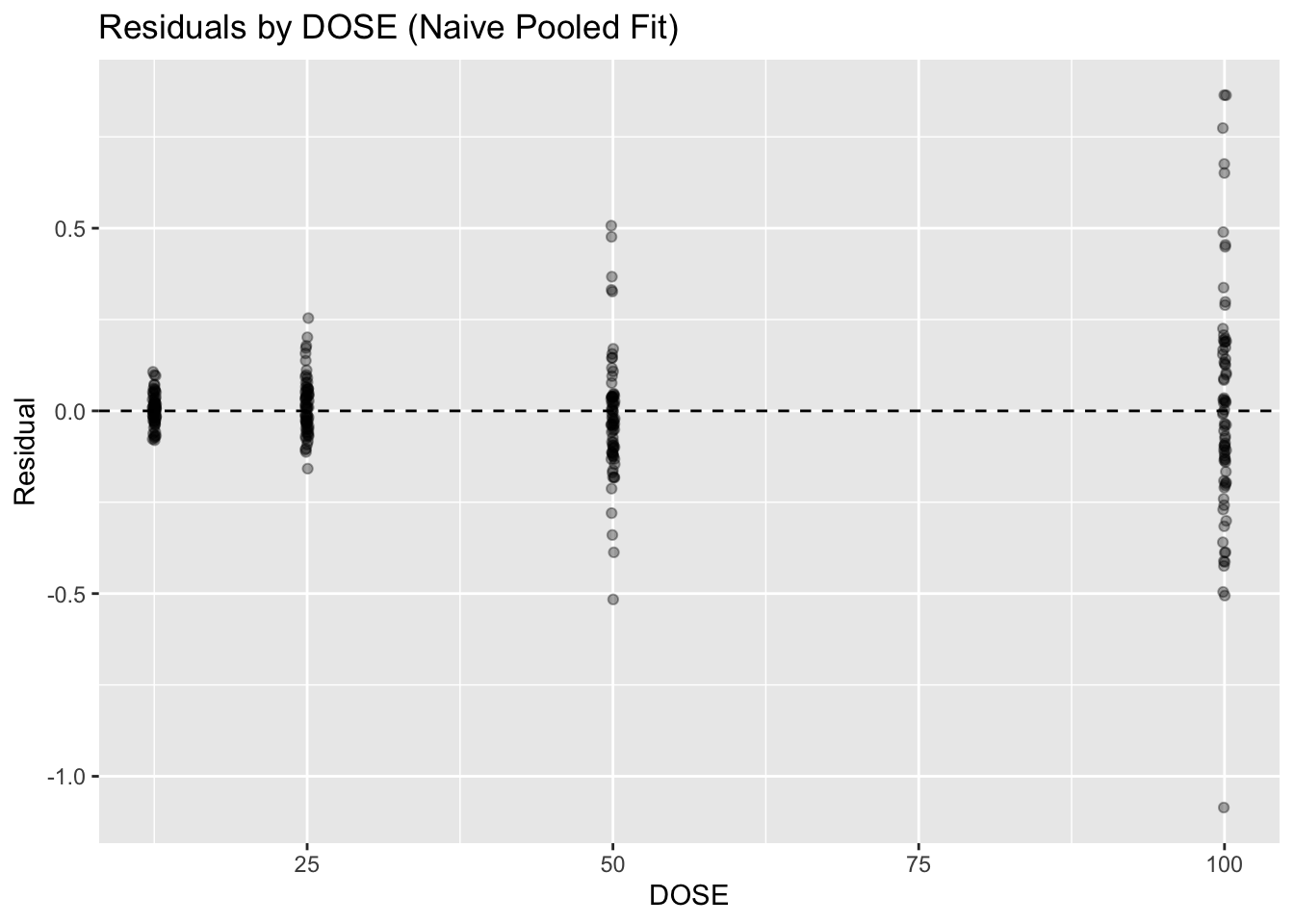
Problem 1: Stratify residuals by DOSE

This checks whether residual magnitude changes with dose. Larger residuals at higher doses can suggest heteroscedasticity, scaling issues, or structural model misspecification.

obs %>%
  group_by(DOSE) %>%
  summarise(
    n = n(),
    rmse = sqrt(mean(residual^2, na.rm = TRUE)),
    median_abs_resid = median(abs(residual), na.rm = TRUE),
    .groups = "drop"
  ) %>%
  arrange(DOSE)

# A tibble: 4 × 4
   DOSE     n   rmse median_abs_resid
  <dbl> <int>  <dbl>            <dbl>
1  12.5    67 0.0428           0.0242
2  25      72 0.0774           0.0478
3  50      74 0.166            0.0854
4 100      76 0.320            0.170

A quick visual:

ggplot(obs, aes(DOSE, residual)) +
  geom_point(alpha = 0.35, position = position_jitter(width = 0.15)) +
  geom_hline(yintercept = 0, linetype = 2) +
  labs(
    title = "Residuals by DOSE (Naive Pooled Fit)",
    x = "DOSE",
    y = "Residual"
  )

Problem 2: Create a log-scale concentration plot

For a log-scale plot, we filter to positive concentrations because scale_y_log10() cannot display zero or negative values.

p_log <- obs %>%
  filter(!is.na(DV) & DV > 0) %>%
  ggplot(aes(TIME, DV, group = ID)) +
  geom_line(alpha = 0.25) +
  geom_point(size = 0.7) +
  facet_wrap(~ DOSE) +
  scale_y_log10() +
  labs(
    title = "Observed Concentration–Time Profiles by DOSE (Log Scale)",
    x = "Time After Dose (h)",
    y = "Concentration (log scale)"
  )

p_log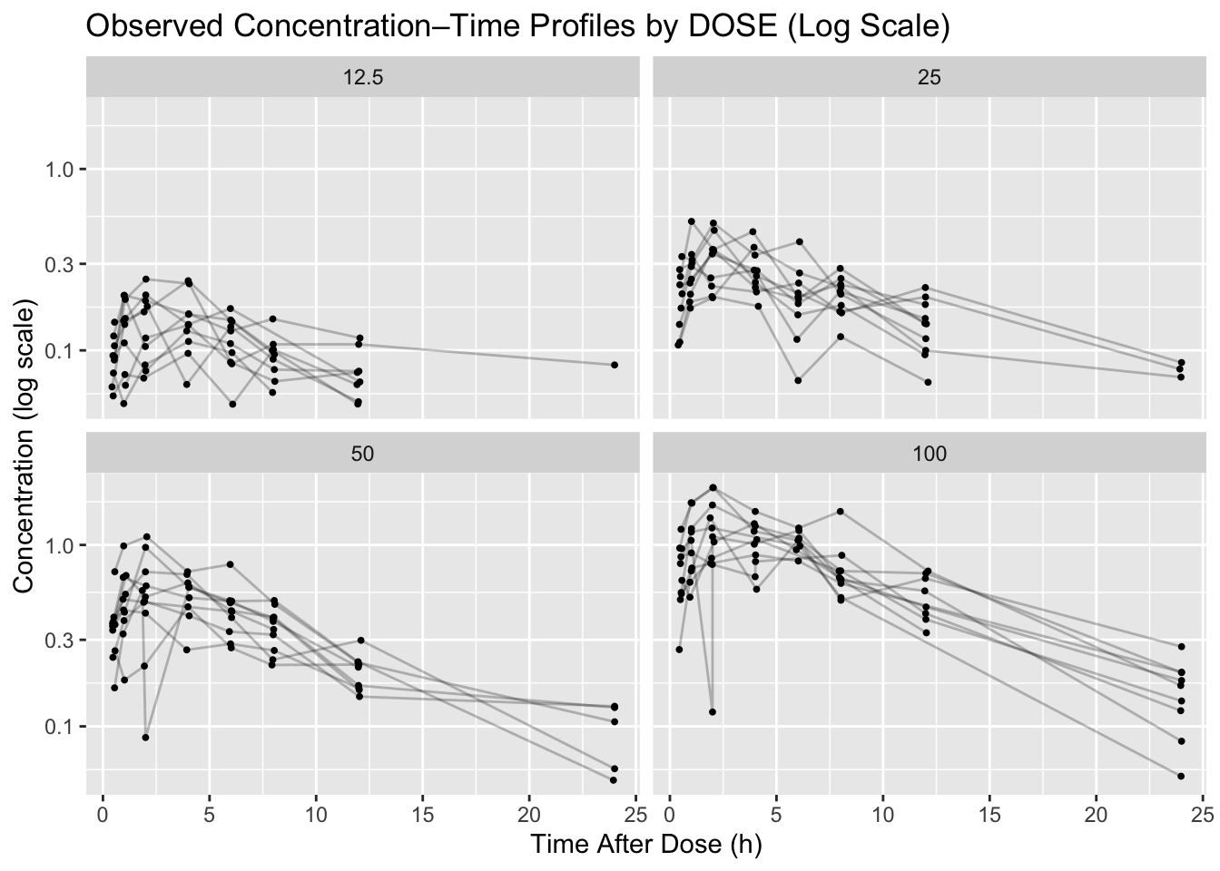

Save it:

ggsave(file.path(resultspath, "profiles_by_dose_log_observed.png"), p_log, width = 9, height = 6)

Problem 3: Compute RMSE of the pooled fit

rmse <- sqrt(mean(obs$residual^2, na.rm = TRUE))
rmse

[1] 0.1895263

You can also compute RMSE by dose, which is often more informative than one pooled value:

obs %>%
  group_by(DOSE) %>%
  summarise(
    rmse = sqrt(mean(residual^2, na.rm = TRUE)),
    .groups = "drop"
  ) %>%
  arrange(DOSE)

# A tibble: 4 × 2
   DOSE   rmse
  <dbl>  <dbl>
1  12.5 0.0428
2  25   0.0774
3  50   0.166 
4 100   0.320

Summary

You fit a one-compartment oral model using naive pooling.
One parameter set describes all subjects.
Dose explains systematic profile differences.
Residual error absorbs inter-individual variability.
This approach is simple but limited.

Quick Tips

Naive pooling is a useful baseline, not a final answer.
Always facet plots by subject to reveal hidden variability.
Large residual spread often signals ignored hierarchy.
CL/V parameterization keeps interpretation physiologically meaningful.
Move to mixed-effects modeling when variability matters.