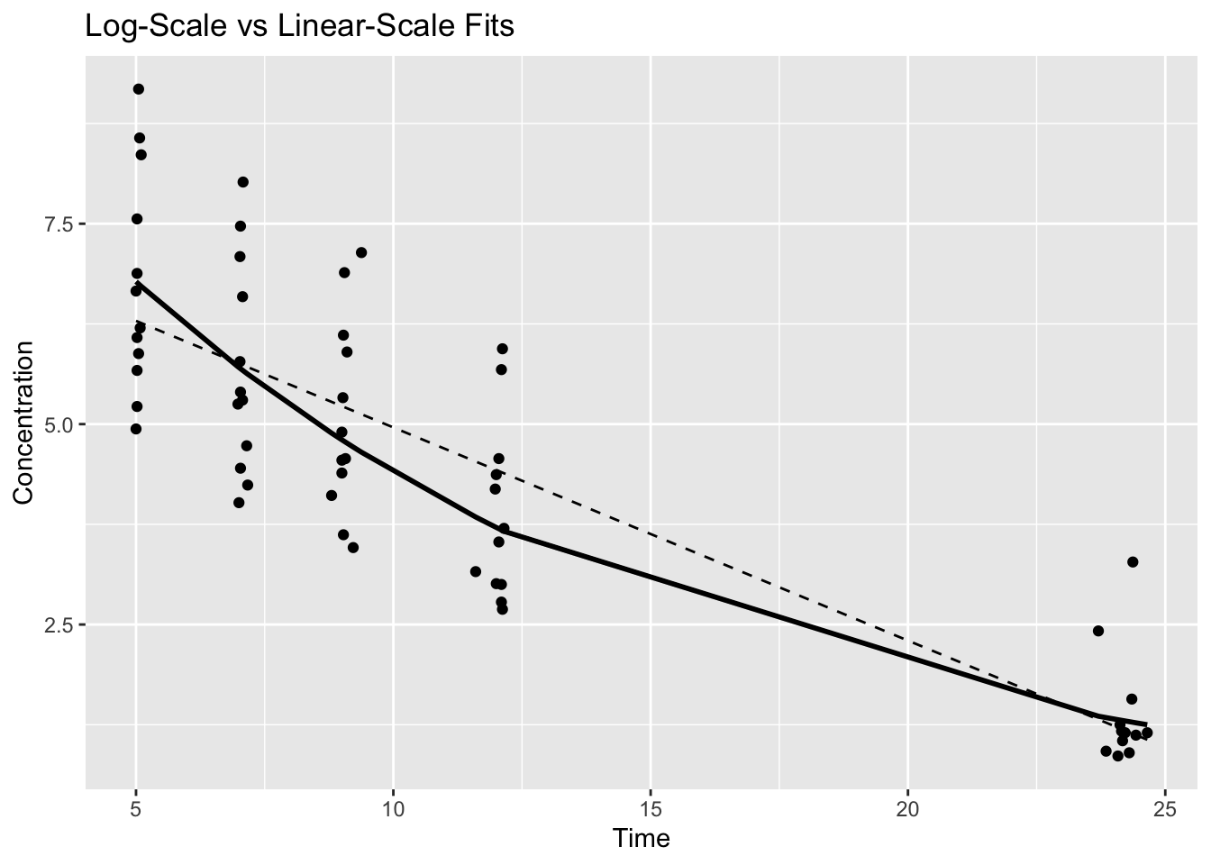
Exponential structure is poorly represented on the original scale.
Worked Example 3: Adding a Covariate (Weight)
lm_cov <-lm(log(conc) ~ Time + Wt, data = terminal_data)summary(lm_cov)
Call:
lm(formula = log(conc) ~ Time + Wt, data = terminal_data)
Residuals:
Min 1Q Median 3Q Max
-0.46733 -0.17124 -0.03331 0.08599 1.03806
Coefficients:
Estimate Std. Error t value Pr(>|t|)
(Intercept) 3.019678 0.263962 11.440 <2e-16 ***
Time -0.086045 0.004937 -17.430 <2e-16 ***
Wt -0.009711 0.003673 -2.644 0.0106 *
---
Signif. codes: 0 '***' 0.001 '**' 0.01 '*' 0.05 '.' 0.1 ' ' 1
Residual standard error: 0.2589 on 57 degrees of freedom
Multiple R-squared: 0.845, Adjusted R-squared: 0.8395
F-statistic: 155.4 on 2 and 57 DF, p-value: < 2.2e-16
anova(lm_fit, lm_cov)
Analysis of Variance Table
Model 1: log(conc) ~ Time
Model 2: log(conc) ~ Time + Wt
Res.Df RSS Df Sum of Sq F Pr(>F)
1 58 4.2878
2 57 3.8194 1 0.46839 6.9902 0.01057 *
---
Signif. codes: 0 '***' 0.001 '**' 0.01 '*' 0.05 '.' 0.1 ' ' 1
Suppose the ANOVA table shows:
p-value ≈ 0.01
Reduced RSS
What This Means (Technically)
Weight explains additional variation in log concentration beyond Time alone.
What This Does Not Mean
It does not prove weight mechanistically alters clearance.
It does not justify inclusion in a population model.
It does not confirm a clinically meaningful effect.
It does not fix the hierarchical assumption violation.
The Critical PMx Perspective
This model:
Treats all observations as independent.
Ignores between-subject variability structure.
Violates core assumptions of independent residuals.
So the p-value is a screening signal, not confirmatory evidence.
A mature conclusion would be:
Weight appears associated with concentration in pooled analysis, but the hierarchical structure of the data is ignored. This motivates mixed-effects modeling rather than formal inference.
That is appropriate scientific restraint.
Worked Example 4: Does Residual Structure Improve?
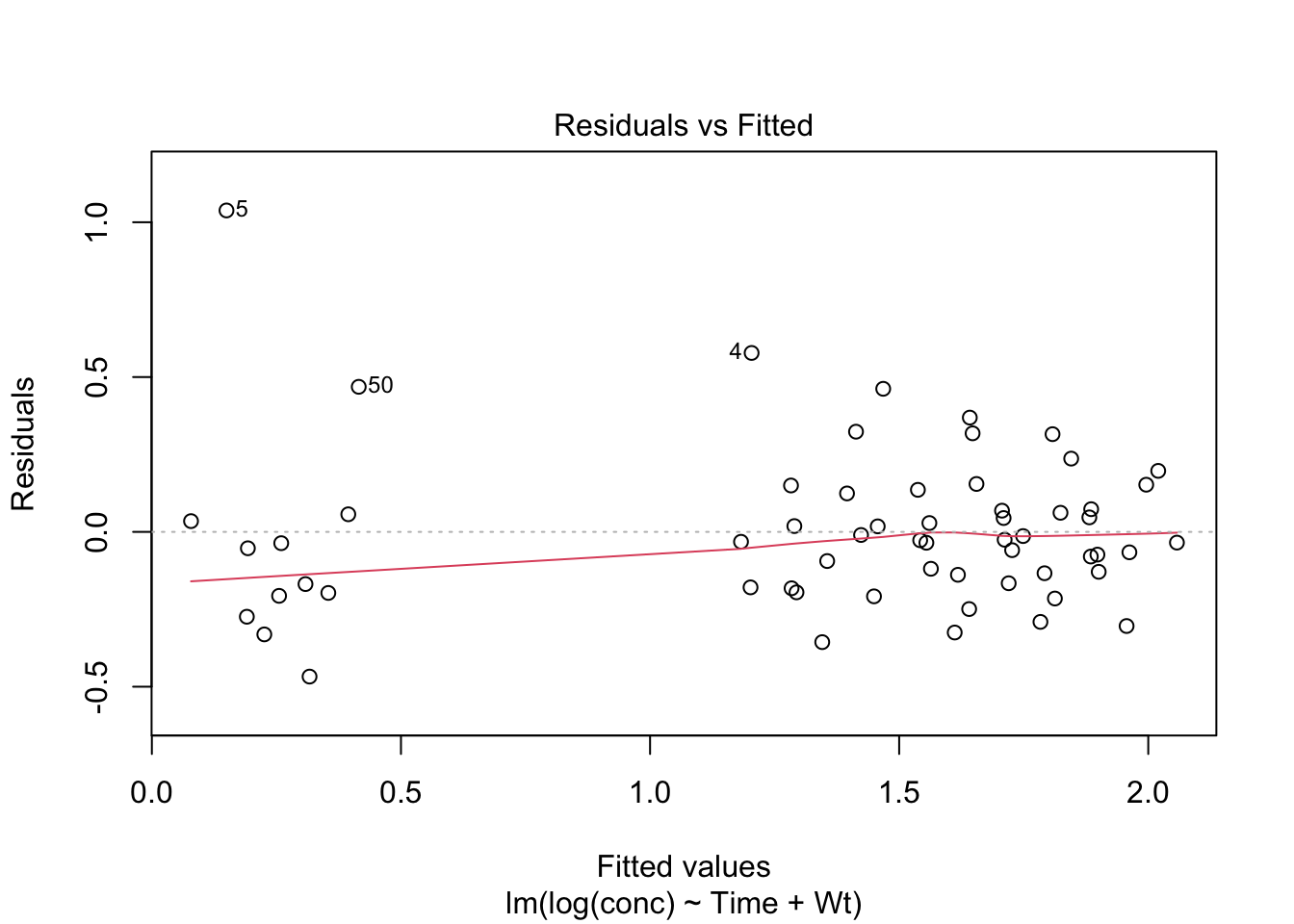
After adding the covariate, inspect residuals:
plot(lm_cov, which =1)
Ask:
Did curvature disappear?
Did variance patterns improve?
Or did we simply reduce RSS slightly?
A useful visual check is whether the residual spread stays roughly constant across fitted values.
For example:
A roughly even vertical spread is usually reassuring
A widening or narrowing “funnel shape” suggests changing variance
This pattern is called heteroscedasticity.
At this stage, the key idea is simple:
The model should not make much larger errors in one region of the data than another.
In pharmacometrics:
Residual structure matters more than p-values.
Strategies
Interpret coefficients in biological units.
Choose scale based on structure, not convenience.
Separate statistical detectability from mechanistic meaning.
Use pooled models for screening, not confirmation.
Common Mistakes
Interpreting statistical significance as mechanistic truth
Fitting PK data on the wrong scale
Forgetting that slopes have biological meaning
Assuming pooled observations are independent
Treating covariate screening as confirmatory analysis
Ignoring residual patterns after fitting the model
Trusting p-values without checking assumptions
Assuming a lower RSS automatically means a better model
Practice Problems
Compute half-life from the fitted slope.
Compare AIC between lm_fit and lm_cov.
Interpret the weight coefficient in biological terms.
Explain why pooled inference is fragile in repeated-measures PK data.
TipStep-by-Step Solutions
Problem 1
ke <--coef(lm_fit)["Time"]log(2)/ke
    Time
8.056956
Problem 2
AIC(lm_fit, lm_cov)
       df      AIC
lm_fit  3 17.95860
lm_cov  4 13.01791
Problem 3
The weight coefficient represents a change in log concentration per kg, not necessarily a change in clearance.
Problem 4
Because repeated measurements within subjects violate independence assumptions.
Summary
Slopes on the log scale approximate elimination rates.
Scale choice encodes structural assumptions.
Covariate significance does not equal mechanistic truth.
Pooled models ignore hierarchy.
Linear modeling is a screening tool before nonlinear and mixed-effects frameworks.
TipQuick Tips
Interpret slopes biologically.
Treat pooled covariate effects as provisional.
Check residual structure before trusting p-values.
Escalate to hierarchical modeling when appropriate.