library(tidyverse)
library(nlme)

data(PBG)

pbg_placebo <- PBG %>%
filter(Treatment == "Placebo")Nonlinear Modeling with nls(): Dose–Response and Saturation
Fitting a Hill (Sigmoid Emax) Model to the PBG Dataset (Placebo Rabbits)
Learning Objectives
By the end of this lesson, you will be able to:
- Recognize when a biological relationship is structurally nonlinear
- Explain why dose–response saturation is not well-captured by a simple line
- Write and interpret a Hill (sigmoid Emax) dose–response model
- Choose reasonable starting values for nonlinear regression
- Fit nonlinear models using
nls()and interpret output meaningfully - Diagnose fragility (start sensitivity) and common failure modes
- Explain why this is structural modeling — not yet population modeling
Key Ideas
- Dose–response saturation is intrinsically nonlinear.
- A Hill model is a sigmoid Emax model: it adds a Hill exponent to control steepness.
- Starting values are part of modeling (they encode your first best guess).
- Convergence is necessary but not sufficient for scientific validity.
- Structural modeling does not account for rabbit-to-rabbit variability unless you explicitly model hierarchy.
Worked Example 1: Visualize the Data (Placebo Only)
We use the PBG dataset from the nlme package.
Each rabbit received increasing doses of phenylbiguanide under placebo or antagonist treatment.
Here we focus on Placebo only to keep the structural question simple.
Plot dose versus change in blood pressure:
ggplot(pbg_placebo, aes(dose, deltaBP, group = Rabbit)) +
  geom_point(size = 2) +
  geom_line(alpha = 0.5) +
  labs(
    title = "Dose–Response (Placebo Rabbits)",
    x = "Dose",
    y = "Change in Blood Pressure"
  )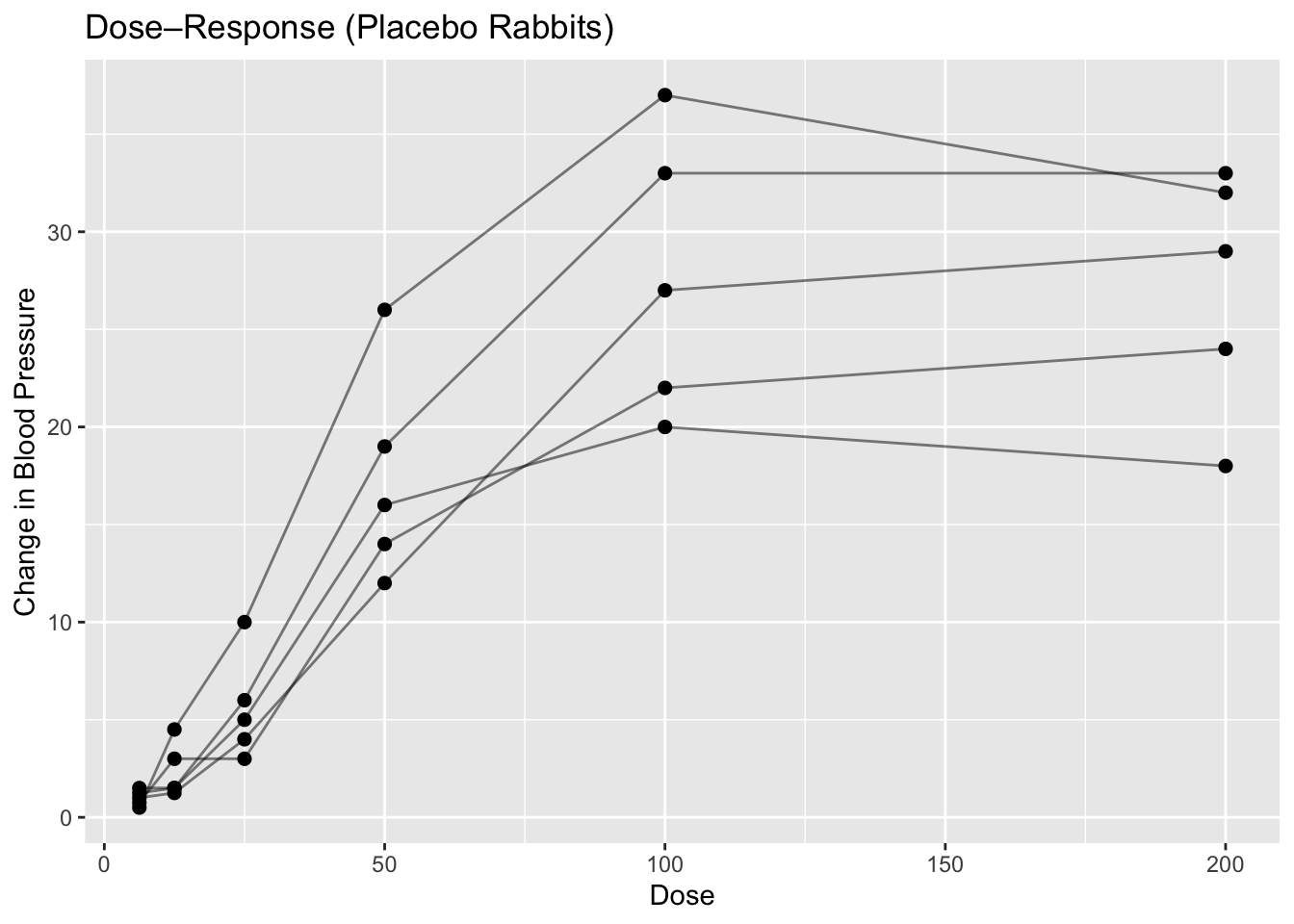
Observe:
- Response increases with dose.
- The curve begins to plateau (saturation).
- Rabbits differ in level, but share a similar shape.
This pattern motivates a nonlinear dose–response model.
Worked Example 2: Why a Linear Model Fails Structurally
A line assumes the effect grows at a constant rate as dose increases.
Try it anyway so you can see the mismatch:
lm_linear <- lm(deltaBP ~ dose, data = pbg_placebo)
summary(lm_linear)
Call:
lm(formula = deltaBP ~ dose, data = pbg_placebo)

Residuals:
    Min      1Q  Median      3Q     Max
-14.761  -4.261  -2.253   2.568  18.529

Coefficients:
            Estimate Std. Error t value Pr(>|t|)
(Intercept)  4.18035    1.83904   2.273   0.0309 *
dose         0.14290    0.01951   7.325 5.63e-08 ***
---
Signif. codes:  0 '***' 0.001 '**' 0.01 '*' 0.05 '.' 0.1 ' ' 1

Residual standard error: 7.231 on 28 degrees of freedom
Multiple R-squared:  0.6571,    Adjusted R-squared:  0.6449
F-statistic: 53.66 on 1 and 28 DF,  p-value: 5.631e-08
Overlay the linear fit:
pbg_placebo %>%
  mutate(pred = predict(lm_linear)) %>%
  ggplot(aes(dose, deltaBP)) +
  geom_point() +
  geom_line(aes(y = pred), linewidth = 1) +
  labs(title = "Linear Fit (Structurally Inadequate)")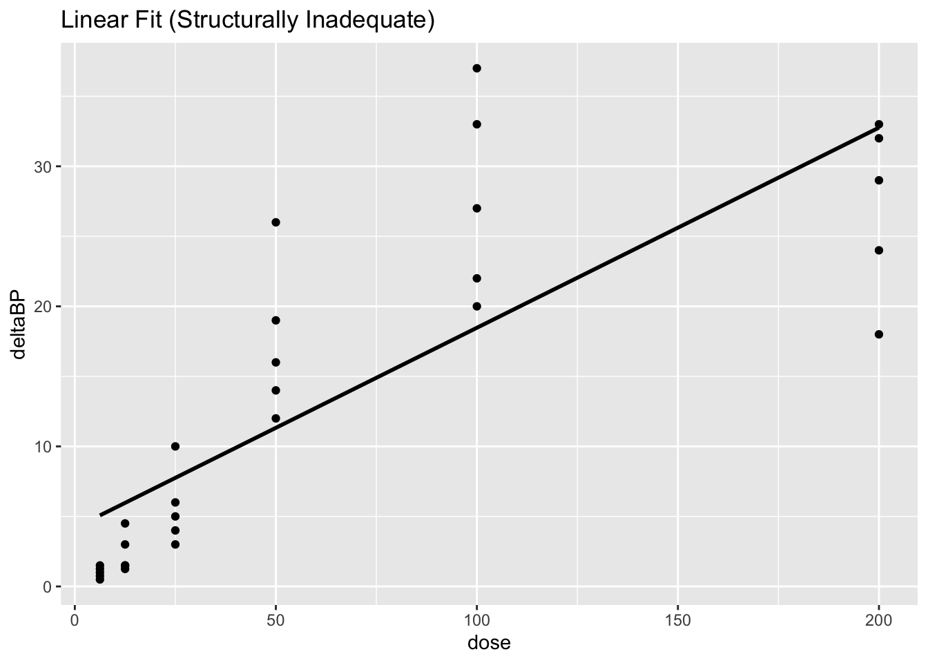
Even if the line looks “okay” in places, it cannot represent a biological plateau.
This is a structural problem, not a “tune the optimizer” problem.
Worked Example 3: The Hill (Sigmoid Emax) Model
A standard Hill model (sigmoid Emax) is:
\[ E(D) = E_0 + \frac{E_{max} \cdot D^{h}}{EC_{50}^{h} + D^{h}} \]
Where:
- \(E_0\) = baseline effect
- \(E_{max}\) = maximum additional effect above baseline
- \(EC_{50}\) = dose producing half of \(E_{max}\) (a potency parameter)
- \(h\) = Hill exponent (controls steepness)
Is this “just Emax with an extra parameter”?
Yes: when \(h = 1\), the Hill model reduces to the classic Emax model.
The Hill exponent is useful when the curve is steeper or shallower than standard Emax.
Worked Example 4: Choose Starting Values (Including Hill)
Starting values should reflect what you see in the plot:
- \(E_0\) ≈ minimum observed response
- \(E_{max}\) ≈ (max − min response)
- \(EC_{50}\) ≈ a mid-range dose (a crude but often workable start)
- \(h\) often starts at 1 (classic Emax), then you let the model adjust
start_vals <- list(
  E0 = min(pbg_placebo$deltaBP),
  Emax = max(pbg_placebo$deltaBP) - min(pbg_placebo$deltaBP),
  EC50 = median(pbg_placebo$dose),
  h = 1
)

start_vals
$E0
[1] 0.5
$Emax
[1] 36.5
$EC50
[1] 37.5
$h
[1] 1
Tip
For Hill models, h and EC50 can trade off (identifiability).
Starting at h = 1 keeps the first fit stable and interpretable.
Worked Example 5: Fit the Hill Model with nls()
fit_hill <- nls(
  deltaBP ~ E0 + (Emax * dose^h) / (EC50^h + dose^h),
  data = pbg_placebo,
  start = start_vals
)

summary(fit_hill)
Formula: deltaBP ~ E0 + (Emax * dose^h)/(EC50^h + dose^h)

Parameters:
     Estimate Std. Error t value Pr(>|t|)
E0      1.549      1.628   0.951  0.35016
Emax   26.697      2.755   9.690 4.07e-10 ***
EC50   43.599      4.910   8.879 2.37e-09 ***
h       3.307      1.175   2.813  0.00922 **
---
Signif. codes:  0 '***' 0.001 '**' 0.01 '*' 0.05 '.' 0.1 ' ' 1

Residual standard error: 4.529 on 26 degrees of freedom

Number of iterations to convergence: 8
Achieved convergence tolerance: 8.882e-06
Interpretation:
- E0: baseline blood pressure change
- Emax: maximum additional increase
- EC50: potency (lower EC50 = more potent)
- h: steepness (higher = steeper transition around EC50)
Worked Example 6: Overlay Model Predictions
Create a smooth dose grid and predict on it:
grid <- tibble(dose = seq(min(pbg_placebo$dose),
                          max(pbg_placebo$dose),
                          length.out = 200)) %>%
  mutate(pred = predict(fit_hill, newdata = .))
Overlay:
ggplot(pbg_placebo, aes(dose, deltaBP)) +
  geom_point(size = 2) +
  geom_line(aes(group = Rabbit), alpha = 0.4) +
  geom_line(
    data = grid,
    aes(dose, pred),
    inherit.aes = FALSE,
    linewidth = 1
  ) +
  labs(title = "Hill (Sigmoid Emax) Fit — Placebo Rabbits")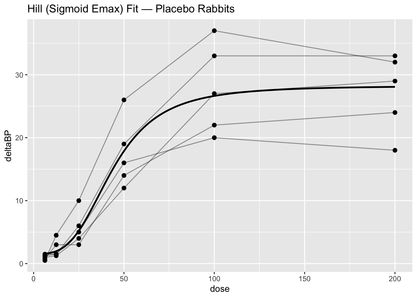
The overlay is your reality check:
- Does the curve capture the plateau?
- Is the steepness plausible?
- Does it systematically miss low or high doses?
Worked Example 7: Sensitivity to Starting Values (and Why It Matters)
Try deliberately poor starting values:
try(
  nls(
    deltaBP ~ E0 + (Emax * dose^h) / (EC50^h + dose^h),
    data = pbg_placebo,
    start = list(E0 = 0, Emax = 1000, EC50 = 0.001, h = 10)
  )
)
Error in nlsModel(formula, mf, start, wts, scaleOffset = scOff, nDcentral = nDcntr) :
singular gradient matrix at initial parameter estimatesNonlinear models may:
- Fail to converge
- Converge to implausible parameters
- Land in a local optimum that “fits” but makes no biological sense
This sensitivity is not a nuisance — it is information about model stability.
Residual Diagnostics
pbg_placebo %>%
  mutate(resid = residuals(fit_hill)) %>%
  ggplot(aes(dose, resid)) +
  geom_point(size = 2) +
  geom_hline(yintercept = 0, linetype = 2) +
  labs(title = "Residuals vs Dose (Hill Model)",
       y = "Residual")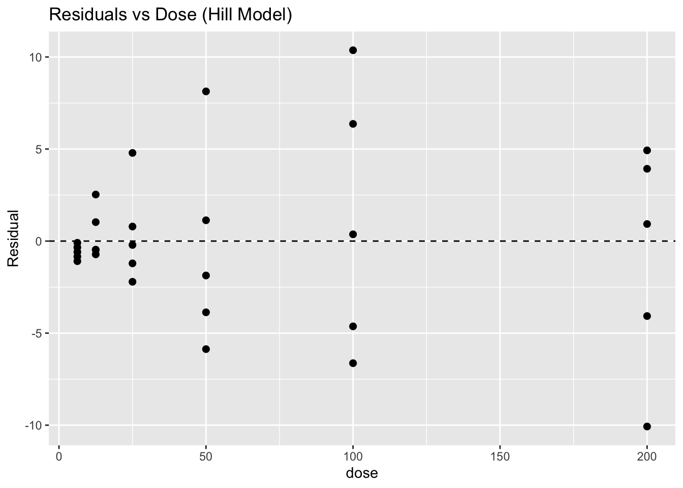
Look for:
- Curvature (still missing structure)
- Dose-dependent variance (error model mismatch)
- Outliers (experimental anomalies or model misspecification)
If the residual spread becomes larger or smaller across the dose range, the model may not be capturing the variability structure correctly.
For example:
- Residuals spreading outward at higher doses create a funnel shape
- Residuals becoming tighter at some doses suggest changing variance
This is another example of heteroscedasticity — the error size changes across the prediction range instead of remaining roughly constant.
What This Model Is — and Is Not
This is:
- Structural nonlinear regression
- A mechanistic approximation of dose–response saturation
This is not:
- A mixed-effects model
- A hierarchical model
- A population PK/PD model
Because we have repeated measures per rabbit, independence is violated.
So treat this as exploratory structure learning — and then escalate to mixed-effects methods.
Strategies
- Always visualize dose–response before fitting.
- Fit one treatment group at a time when exploring structure.
- Use plots to estimate starting values.
- Overlay predictions to verify plausibility.
- Interpret parameters biologically (E0, Emax, EC50, Hill), not just numerically.
Common Mistakes
- Fitting a straight line to a saturating relationship
- Choosing arbitrary starting values without looking at the data
- Assuming convergence means the model is correct
- Ignoring implausible parameter estimates after fitting
- Interpreting EC50 without understanding potency
- Treating the Hill exponent as “just another parameter”
- Forgetting that repeated measures violate independence
- Trusting the fit without checking overlays or residuals
Practice Problems
- Extract parameter estimates using
coef(). - Compute predicted response at dose = 5 using
predict(newdata=...). - Refit with starting values
h = 1,h = 2, andh = 0.5. Compare results. - In one sentence, explain why rabbit-level repeated measures motivate mixed-effects modeling.
TipStep-by-Step Solutions
Problem 1
coef(fit_hill) E0 Emax EC50 h
1.548753 26.696588 43.598902 3.306525 Problem 2
predict(fit_hill, newdata = data.frame(dose = 5))[1] 1.569469Problem 3
fit_h1 <- nls(
  deltaBP ~ E0 + (Emax * dose^h) / (EC50^h + dose^h),
  data = pbg_placebo,
  start = list(
    E0 = min(pbg_placebo$deltaBP),
    Emax = max(pbg_placebo$deltaBP) - min(pbg_placebo$deltaBP),
    EC50 = median(pbg_placebo$dose),
    h = 1
  )
)

fit_h2 <- nls(
  deltaBP ~ E0 + (Emax * dose^h) / (EC50^h + dose^h),
  data = pbg_placebo,
  start = list(
    E0 = min(pbg_placebo$deltaBP),
    Emax = max(pbg_placebo$deltaBP) - min(pbg_placebo$deltaBP),
    EC50 = median(pbg_placebo$dose),
    h = 2
  )
)

fit_h05 <- nls(
  deltaBP ~ E0 + (Emax * dose^h) / (EC50^h + dose^h),
  data = pbg_placebo,
  start = list(
    E0 = min(pbg_placebo$deltaBP),
    Emax = max(pbg_placebo$deltaBP) - min(pbg_placebo$deltaBP),
    EC50 = median(pbg_placebo$dose),
    h = 0.5
  )
)

coef(fit_h1)
E0 Emax EC50 h
1.548753 26.696588 43.598902 3.306525 coef(fit_h2) E0 Emax EC50 h
1.548752 26.696576 43.598858 3.306531 coef(fit_h05) E0 Emax EC50 h
1.548763 26.696546 43.598839 3.306548 If results vary wildly across starts, treat the Hill fit as fragile.
Problem 4
Because multiple measurements per rabbit create within-rabbit dependence that pooled nls() does not model.
Summary
- Dose–response saturation is structurally nonlinear.
- The Hill model generalizes Emax by adding a steepness parameter (\(h\)).
- Starting values are part of the modeling workflow.
- Convergence is not proof of correctness — overlays and residuals matter.
- Hierarchical modeling is the natural next step for repeated-measures dose–response data.
TipQuick Tips
- Plot dose–response before fitting.
- Start with h = 1 (classic Emax) for stability.
- Always overlay predictions on the observed data.
- If h and EC50 are unstable, simplify or move to a hierarchical framework.