library(tidyverse)
library(nlmixr2data)

data(
  "theo_sd",
  package = "nlmixr2data"
)Exploring Covariates Visually
Use exploratory visualization to identify possible covariate relationships before building covariate models.
Tip
Big picture: Covariate modeling starts with understanding the data—not fitting equations.
Learning Objectives
By the end of this lesson, you will be able to:
- explain why covariate exploration matters
- distinguish continuous and categorical covariates
- visualize covariate relationships
- recognize useful exploratory patterns
- identify candidate covariates before model building
Key Ideas
- visualize before modeling
- trends matter more than individual points
- biology guides interpretation
- exploration does not prove causality
Setup
Create example covariates for exploration.
set.seed(100)

cov_tbl <-
  theo_sd %>%
  distinct(ID, WT) %>%
  mutate(
    SEX = sample(c("F", "M"), n(), replace = TRUE),
    AGE = round(rnorm(n(), mean = 35, sd = 10))
  )
Why Explore Covariates?
Suppose we observe variability.
Question:
Can we explain it?Before building a model:
Visualize → Hypothesize → ModelVisualization helps generate candidate explanations.
Continuous vs Categorical Covariates
Covariates are often grouped into two broad types.
| Type | Description | Examples |
|---|---|---|
| Continuous | Can take many numerical values along a scale | WT, AGE |
| Categorical | Represent groups or categories | SEX, RACE, FORMULATION |
Continuous covariates are usually visualized using scatterplots, histograms, or density plots.
Categorical covariates are often visualized using bar charts or boxplots.
Both types may help explain variability between individuals.
Worked Example 1: Continuous Covariates
Inspect weight.
ggplot(cov_tbl, aes(WT)) +
    geom_histogram(bins = 20) +
    labs(
        title = "Weight Distribution",
        x = "Weight",
        y = "Count"
    )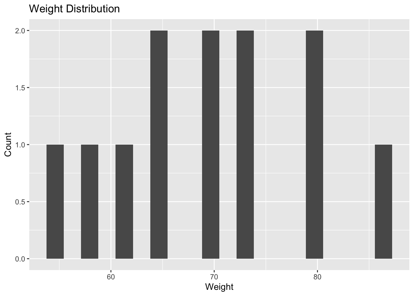
Interpretation:
Ask:
- realistic values?
- broad range?
- possible outliers?
Covariates with little variation often contribute less information.
Worked Example 2: Categorical Covariates
Inspect sex.
ggplot(cov_tbl, aes(SEX)) +
    geom_bar() +
    labs(title = "Sex Distribution",
         x = "Sex",
         y = "Count")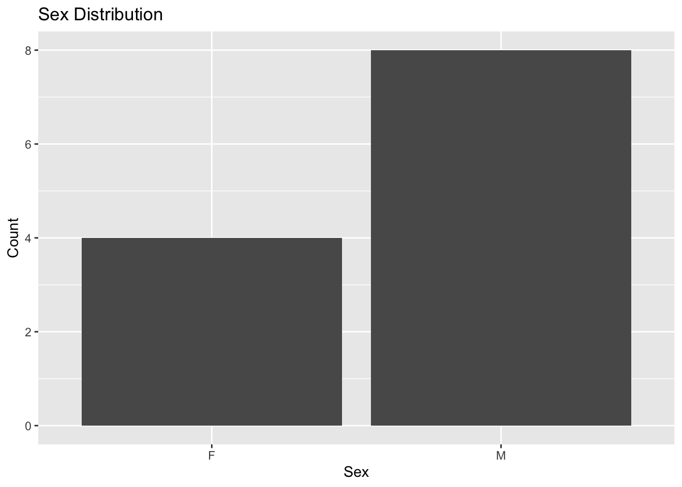
Interpretation:
Ask:
- balanced groups?
- enough observations?
Categorical covariates require representation across groups.
Worked Example 3: Explore Relationships Between Covariates
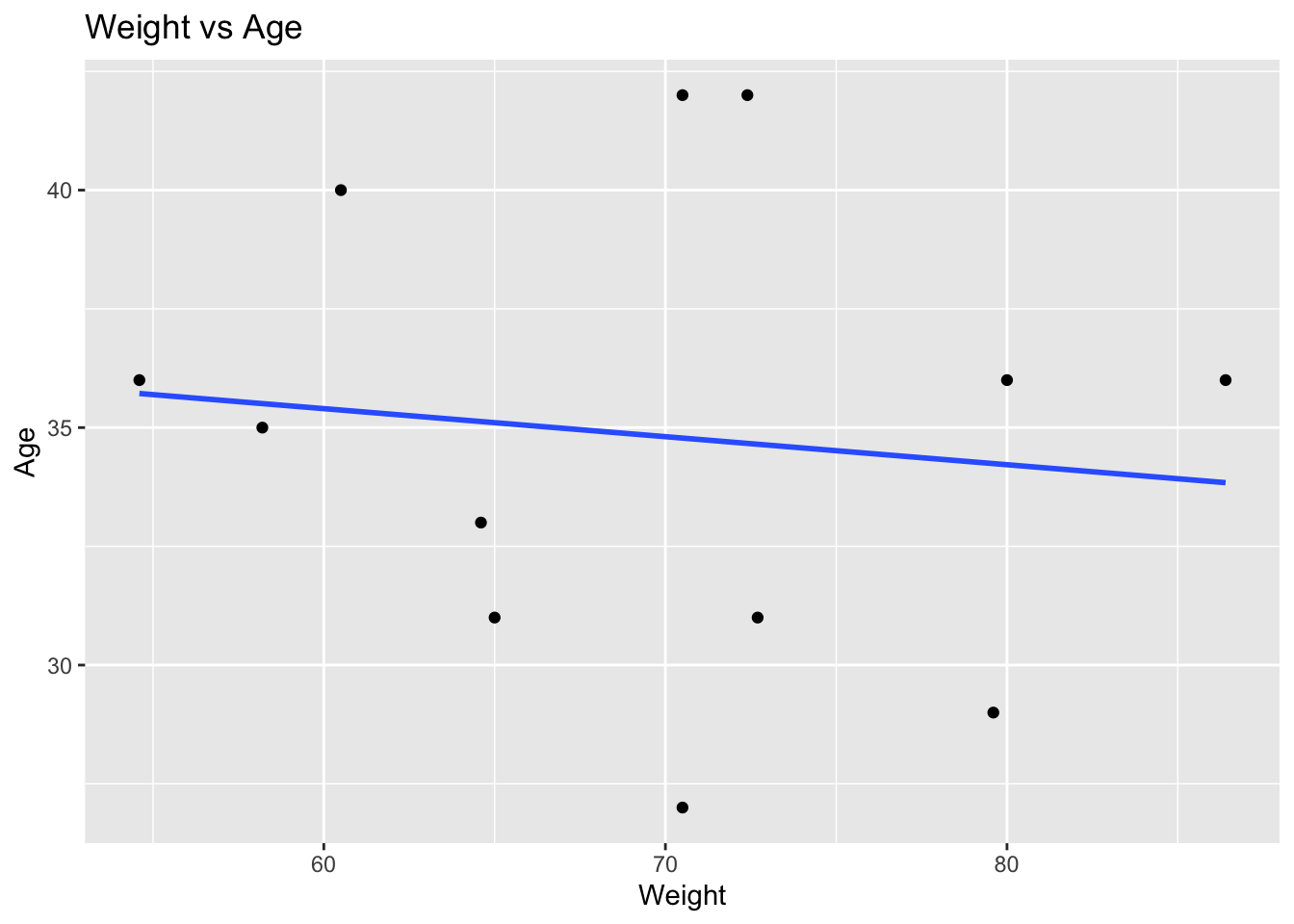
Visualize weight versus age.
ggplot(cov_tbl, aes(WT, AGE)) +
  geom_point() +
  geom_smooth(
    method = "lm",
    se = FALSE
  ) +
  labs(
    title = "Weight vs Age",
    x = "Weight",
    y = "Age"
  )
Interpretation:
Ask:
- is there a visible trend?
- are the points widely scattered?
- do any unusual observations stand out?
Exploratory plots help us understand how variables are distributed and whether relationships might exist.
They generate hypotheses.
They do not prove relationships.
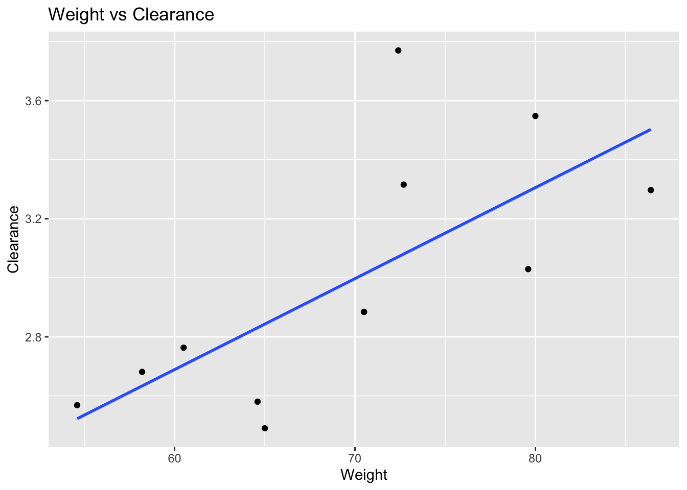
Worked Example 4: Simulate a Candidate Relationship
Create a simple simulated relationship.
cov_effect <-
cov_tbl %>%
    mutate(CL = 3 *(WT / 70)^0.75 + rnorm(n(), 0, 0.3))

ggplot(
  cov_effect, aes(WT, CL)
) +
geom_point() +
geom_smooth(
  method = "lm",
  se = FALSE
) +
labs(
  title = "Weight vs Clearance",
  x = "Weight",
  y = "Clearance"
)
Interpretation:
Possible observations:
- upward trend
- no trend
- large scatter
Patterns generate hypotheses.
Not conclusions.
Worked Example 5: What Makes a Good Covariate?
Candidate covariates should be:
- biologically plausible
- measurable
- interpretable
- supported visually
Avoid selecting covariates only because they appear statistically significant.
Covariates Do Not Prove Causality
A relationship may appear because of:
- confounding
- study design
- sampling
- random variation
Visualization is the beginning.
Not the end.
Looking Ahead
We now have:
Variability → Visualization → Candidate CovariateNext we ask:
How do we incorporate covariates into an
nlmixr2model?
Strategies
- visualize first
- think mechanistically
- look for broad patterns
Common Mistakes
- overinterpreting scatter
- selecting every relationship
- ignoring study design
Practice Problems
Why explore covariates before modeling?
Give one continuous and one categorical covariate.
What pattern would suggest a possible relationship?
Why is visualization not enough?
What makes a good covariate?
TipStep-by-Step Solutions
Problem 1
Exploration generates hypotheses.
Problem 2
Examples:
Continuous:
- weight
Categorical:
- sex
Problem 3
Consistent directional behavior may suggest a relationship.
Problem 4
Visualization does not establish mechanism.
Problem 5
Good covariates are:
- biologically meaningful
- measurable
- interpretable
Summary
- covariate modeling begins with exploration
- patterns generate hypotheses
- biology matters
- visualization precedes modeling
TipQuick Tips
- Visualize first
- Trends > points
- Biology first
- Correlation ≠ causation