library(tidyverse)
library(rxode2)Exploring Dose Scenarios
Use simulation to compare doses and dosing schedules and understand exposure changes.
Tip
Big picture: Simulation becomes powerful when we compare treatment strategies rather than describing a single outcome.
Learning Objectives
By the end of this lesson, you will be able to:
- compare alternative dose scenarios
- simulate different dosing schedules
- interpret exposure changes
- distinguish dose and schedule effects
- connect simulation to decision making
Key Ideas
- simulation supports scenario comparison
- dose changes alter exposure
- schedules alter timing
- outcomes should be interpreted in context
Setup
This lesson uses simulation only.
No estimation is performed.
Why Compare Dose Scenarios?
Once a model exists, we can ask:
- what if dose increases?
- what if dose decreases?
- what if dosing becomes more frequent?
- what if concentration accumulates?
Simulation helps answer these questions before collecting new data.
Conceptually:
Model

↓

Alternative Scenarios

↓

Compare Outcomes
Worked Example 1: Define the Base PK Model
Use the same simple PK model.
pk_model <-
  rxode2({

    ka <- 1
    cl <- 3
    v <- 30

    d/dt(depot) = -ka * depot
    d/dt(center) = ka * depot - cl / v * center

    cp = center / v

  })
Worked Example 2: Compare Dose Levels
Create two scenarios.
ev_100 <-
  et(amt = 100, cmt = "depot") %>%
  et(seq(0, 24, by = 0.25))

ev_200 <-
  et(amt = 200, cmt = "depot") %>%
  et(seq(0, 24, by = 0.25))
Simulate.
sim_100 <-
  rxSolve(pk_model, ev_100) %>%
  as_tibble() %>%
  mutate(DOSE = "100 mg")

sim_200 <-
  rxSolve(pk_model, ev_200) %>%
  as_tibble() %>%
  mutate(DOSE = "200 mg")
Combine.
dose_compare <-
  bind_rows(
    sim_100,
    sim_200
  )
Plot.
ggplot(
  dose_compare,
  aes(
    time,
    cp,
    linetype = DOSE
  )
) +
geom_line() +
labs(
    title = "Effect of Dose",
    x = "Time",
    y = "Concentration"
)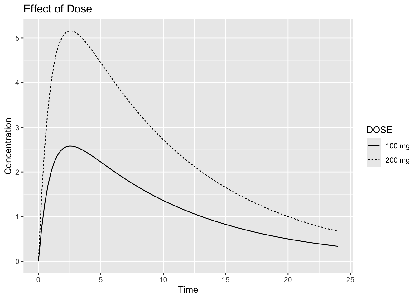
Interpretation:
Ask:
Does doubling dose double exposure?For this simple linear PK model, exposure is expected to increase approximately in proportion to dose.
More complex models may not behave this way.
Notice:
- peak concentration changes
- overall exposure changes
- profile shape may remain similar
Worked Example 3: Compare Dosing Schedules
In the previous example we changed dose.
Now we keep overall daily dose similar and change only the dosing schedule.
100 mg every 24 hours
=
50 mg every 12 hours
=
100 mg/day
Create scenarios.
ev_q24 <-
  et(
    amt = 100,
    ii = 24,
    addl = 4,
    cmt = "depot"
  ) %>%
  et(
    seq(0, 120, by = 0.5)
  )

ev_q24
── EventTable with 242 records ──
1 dosing records (see x$get.dosing(); add with add.dosing or et)
241 observation times (see x$get.sampling(); add with add.sampling or et)
multiple doses in `addl` columns, expand with x$expand(); or etExpand(x)
── First part of x: ──
# A tibble: 242 × 6
time cmt amt ii addl evid
<dbl> <chr> <dbl> <dbl> <int> <evid>
1 0 depot 100 24 4 1:Dose (Add)
2 0 <NA> NA NA NA 0:Observation
3 0.5 <NA> NA NA NA 0:Observation
4 1 <NA> NA NA NA 0:Observation
5 1.5 <NA> NA NA NA 0:Observation
6 2 <NA> NA NA NA 0:Observation
7 2.5 <NA> NA NA NA 0:Observation
8 3 <NA> NA NA NA 0:Observation
9 3.5 <NA> NA NA NA 0:Observation
10 4 <NA> NA NA NA 0:Observation
# ℹ 232 more rowsThe event table now includes additional dosing instructions.
Key arguments:
ii   = interdose interval
addl = additional doses
For example:
amt = 100
ii = 24
addl = 4
means:
100 mg at time 0
100 mg at 24 h
100 mg at 48 h
100 mg at 72 h
100 mg at 96 h
for a total of five doses.
ev_q12 <-
  et(
    amt = 50,
    ii = 12,
    addl = 9,
    cmt = "depot"
  ) %>%
  et(
    seq(0, 120, by = 0.5)
  )

ev_q12
── EventTable with 242 records ──
1 dosing records (see x$get.dosing(); add with add.dosing or et)
241 observation times (see x$get.sampling(); add with add.sampling or et)
multiple doses in `addl` columns, expand with x$expand(); or etExpand(x)
── First part of x: ──
# A tibble: 242 × 6
time cmt amt ii addl evid
<dbl> <chr> <dbl> <dbl> <int> <evid>
1 0 depot 50 12 9 1:Dose (Add)
2 0 <NA> NA NA NA 0:Observation
3 0.5 <NA> NA NA NA 0:Observation
4 1 <NA> NA NA NA 0:Observation
5 1.5 <NA> NA NA NA 0:Observation
6 2 <NA> NA NA NA 0:Observation
7 2.5 <NA> NA NA NA 0:Observation
8 3 <NA> NA NA NA 0:Observation
9 3.5 <NA> NA NA NA 0:Observation
10 4 <NA> NA NA NA 0:Observation
# ℹ 232 more rowsThese scenarios have the same total daily dose:
This allows us to isolate the effect of dosing schedule while keeping overall daily dose similar.
Simulate.
sim_q24 <-
  rxSolve(pk_model, ev_q24) %>%
  as_tibble() %>%
  mutate(SCHEDULE = "100 mg q24h")

sim_q12 <-
  rxSolve(pk_model, ev_q12) %>%
  as_tibble() %>%
  mutate(SCHEDULE = "50 mg q12h")
Combine.
schedule_compare <-
  bind_rows(
    sim_q24,
    sim_q12
  )
Because doses are repeated before the drug is fully eliminated, concentrations from successive doses may accumulate.
Accumulation is often easier to visualize than to calculate, making simulation particularly useful.
Plot.
ggplot(
  schedule_compare,
  aes(
    time,
    cp,
    linetype = SCHEDULE
  )
) +
geom_line() +
labs(
    title = "Effect of Schedule",
    x = "Time",
    y = "Concentration"
)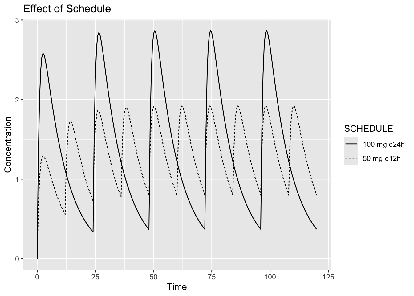
Interpretation:
Compare:
- peak concentration
- trough concentration
- accumulation
Question:
Can the same total daily dose produce different profiles?Yes.
Timing matters.
Worked Example 4: Quantify Exposure
Compute summary measures.
schedule_compare %>%
  group_by(SCHEDULE) %>%
  summarise(
    CMAX = max(cp),
    CMIN = min(cp),
    .groups = "drop"
  )
# A tibble: 2 × 3
SCHEDULE CMAX CMIN
<chr> <dbl> <dbl>
1 100 mg q24h 2.87 0
2 50 mg q12h 1.92 0For simplicity, we compute a few basic summary measures.
In practice, pharmacometric analyses often examine metrics such as:
Cmax

AUC

Trough

Time Above Threshold
Visualization and summaries often complement each other.
Worked Example 5: Scenario Thinking
Simulation does not identify the best treatment.
It compares assumptions.
Conceptually:
Scenario A

↓

Outcome A


Scenario B

↓

Outcome B
Decision making still requires:
- objectives
- safety
- clinical interpretation
Simulation supports decisions.
It does not replace them.
Connecting to Practice
Scenario exploration is common in:
- dose selection
- schedule evaluation
- pediatric extrapolation
- clinical planning
Simulation allows exploration without new experiments.
Looking Ahead
So far we manually defined scenarios.
Next we simulate directly from fitted population models.
Strategies
- compare one change at a time
- visualize profiles
- summarize outcomes
Common Mistakes
- assuming more dose always improves outcomes
- ignoring timing
- overinterpreting simulations
Practice Problems
Why compare scenarios?
What changes when dose changes?
What changes when schedule changes?
Can equal daily dose produce different profiles?
Why summarize simulations?
TipStep-by-Step Solutions
Problem 1
To compare possible outcomes.
Problem 2
Exposure changes.
Problem 3
Timing and accumulation.
Problem 4
Yes.
Schedule matters.
Problem 5
Summaries simplify interpretation.
Summary
- simulation supports comparison
- dose changes exposure
- schedules change timing
- interpretation guides decisions
TipQuick Tips
- Compare fairly
- Change one thing at a time
- Visualize before concluding