Predictions and Residuals

Extract and interpret predictions and residual quantities from the first population PK model.

Tip

Big picture: Predictions connect estimated parameters back to concentration-time behavior. Residuals quantify disagreement and introduce the idea of unexplained variation.

Learning Objectives

By the end of this lesson, you will be able to:

• Extract predictions from an nlmixr2 fit.
• Distinguish PRED and IPRED.
• Understand residual concepts.
• Visualize observed versus predicted values.
• Recognize that residual quantities are generated automatically.

---

Key Ideas

• Predictions are generated from estimated parameters.
• Population and individual predictions differ.
• Residuals quantify disagreement.
• Residuals depend on the model assumptions.

---

Setup

library(tidyverse)
library(nlmixr2)
library(nlmixr2data)

data("theo_sd", package = "nlmixr2data")

Fit the model.

one_comp_model <- function(){

  ini({

    tka <- log(1)

    tcl <- log(3)

    tv <- log(30)

    eta.ka ~ 0.1
    eta.cl ~ 0.1
    eta.v ~ 0.1

    add.err <- 0.1

  })

  model({

    ka <- exp(tka + eta.ka)

    cl <- exp(tcl + eta.cl)

    v <- exp(tv + eta.v)

    linCmt() ~ add(add.err)

  })

}

fit <-
  nlmixr2(
    one_comp_model,
    theo_sd,
    est = "focei",
    control = list(
      print = 0
    )
  )

fit_tbl <- fit %>% as_tibble()

---

Why Predictions Matter

Estimation gives parameter estimates.

Predictions answer:

What concentrations does the model expect?

Residuals answer:

How different are observations from predictions?

Predictions connect:

Estimated Parameters

↓

Expected Concentrations

Residuals connect:

Observed

↓

Predicted

↓

Disagreement

---

Worked Example 1: Explore Prediction Variables

Inspect available variables.

names(fit_tbl)

 [1] "ID"      "TIME"    "DV"      "PRED"    "RES"     "WRES"    "IPRED"  
 [8] "IRES"    "IWRES"   "CPRED"   "CRES"    "CWRES"   "eta.ka"  "eta.cl" 
[15] "eta.v"   "depot"   "central" "ka"      "cl"      "v"       "tad"    
[22] "dosenum"

Common variables include:

Variable	Meaning
DV	observed concentration
PRED	population prediction
IPRED	individual prediction

These variables represent different views of model behavior.

---

Worked Example 2: Population Prediction

Visualize observed versus population prediction.

ggplot(
  fit_tbl,
  aes(PRED, DV)
) +
geom_point(
  alpha = 0.35
) +
geom_abline(
  slope = 1,
  intercept = 0,
  linetype = 2
) +
labs(
  title = "Observed vs Population Prediction",
  x = "PRED",
  y = "DV"
)

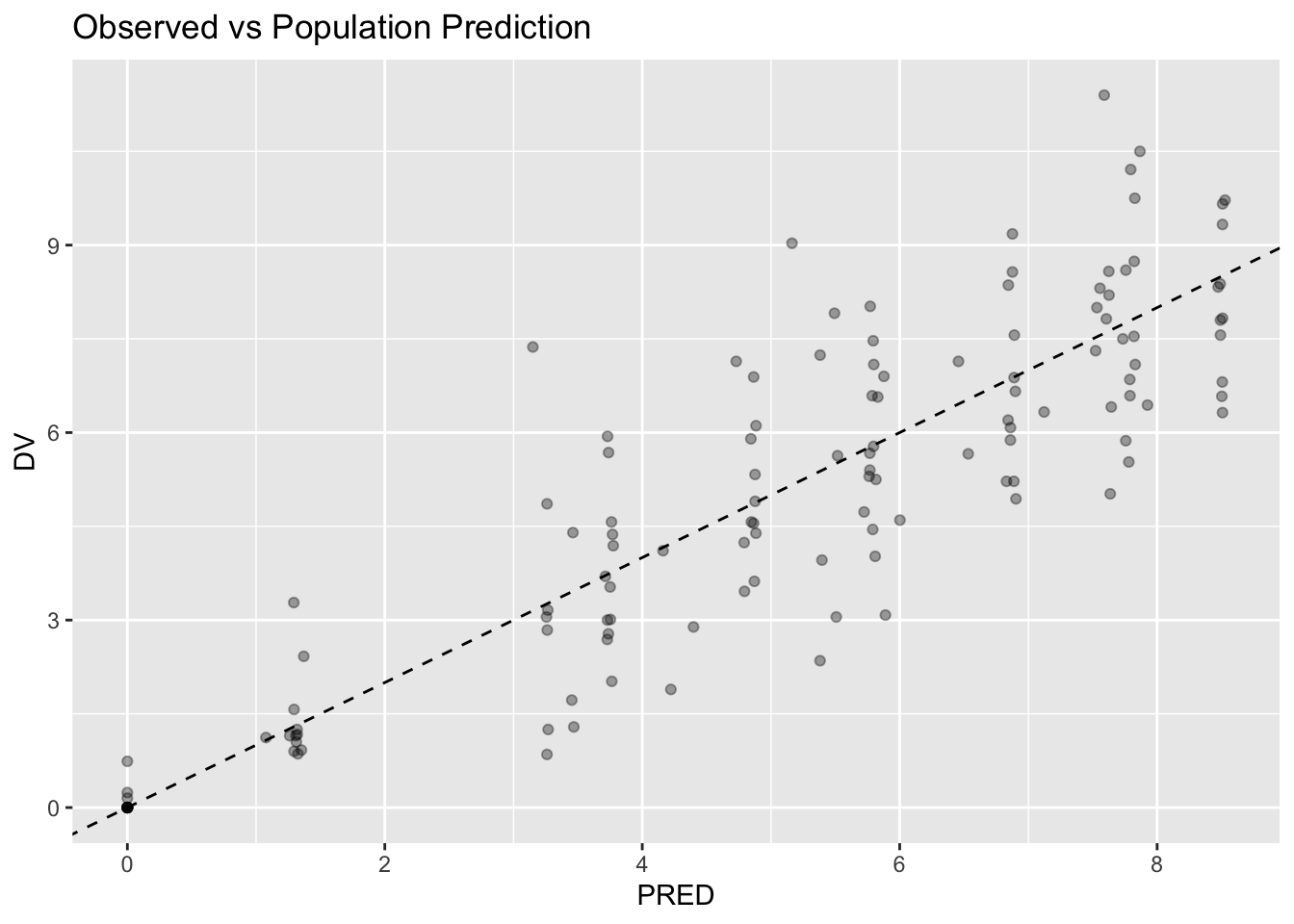
Interpretation:

Population predictions represent expected behavior for the typical subject.

Conceptually:

Typical Parameters

↓

Prediction

---

Worked Example 3: Individual Prediction

Visualize individual predictions.

ggplot(
  fit_tbl,
  aes(IPRED, DV)
) +
geom_point(
  alpha = 0.35
) +
geom_abline(
  slope = 1,
  intercept = 0,
  linetype = 2
) +
labs(
  title = "Observed vs Individual Prediction",
  x = "IPRED",
  y = "DV"
)

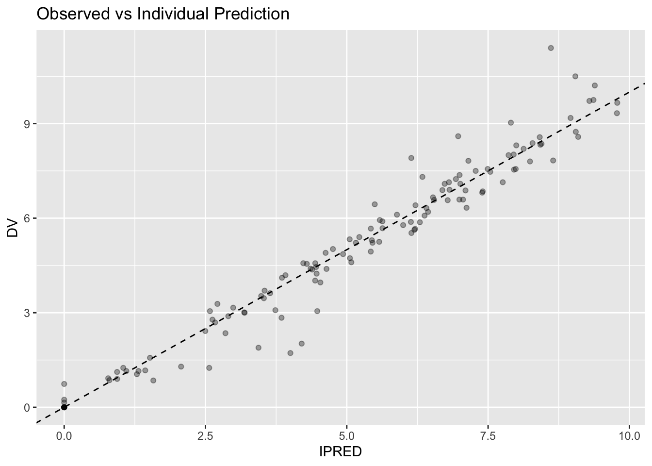
Interpretation:

Individual predictions include subject information.

Conceptually:

Typical Parameters

+

Individual Effects

↓

Prediction

Individual predictions often appear closer to observations.

---

Worked Example 4: Inspect Residual Quantities

Inspect residual quantities already stored in the fit object.

fit_tbl %>%
  select(
    ID,
    TIME,
    DV,
    PRED,
    IPRED,
    RES,
    IRES
  )

# A tibble: 132 × 7
   ID     TIME    DV  PRED IPRED    RES    IRES
   <fct> <dbl> <dbl> <dbl> <dbl>  <dbl>   <dbl>
 1 1      0     0.74  0     0     0.74   0.74  
 2 1      0.25  2.84  3.26  3.85 -0.422 -1.01  
 3 1      0.57  6.57  5.83  6.78  0.740 -0.215 
 4 1      1.12 10.5   7.87  9.04  2.63   1.46  
 5 1      2.02  9.66  8.51  9.79  1.15  -0.125 
 6 1      3.82  8.58  7.62  9.09  0.955 -0.514 
 7 1      5.1   8.36  6.84  8.45  1.52  -0.0853
 8 1      7.03  7.47  5.79  7.54  1.68  -0.0682
 9 1      9.05  6.89  4.87  6.69  2.02   0.198 
10 1     12.1   5.94  3.73  5.58  2.21   0.356 
# ℹ 122 more rows

Interpretation:

DV
Observed

PRED
Population Prediction

IPRED
Individual Prediction

RES
Observed − Population Prediction

IRES
Observed − Individual Prediction

Positive residual:

Observed > Predicted

Negative residual:

Observed < Predicted

These quantities are generated automatically.

No manual residual calculation is needed.

---

Worked Example 5: Visualize Residual Behavior

Plot residuals.

ggplot(
  fit_tbl,
  aes(PRED, RES)
) +
geom_point(
  alpha = 0.35
) +
geom_hline(
  yintercept = 0,
  linetype = 2
) +
labs(
  title = "Residuals vs Population Prediction",
  x = "PRED",
  y = "RES"
)

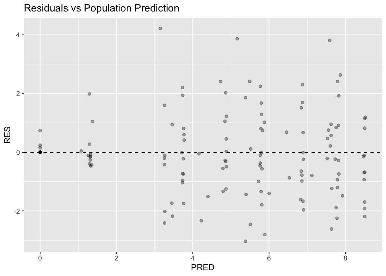
Interpretation:

For now, look for:

• approximate centering around zero
• similar spread
• absence of obvious patterns

Do not draw conclusions yet.

This plot introduces residual thinking.

Formal diagnostic interpretation comes later.

---

Residuals and Error

Residual quantities reflect disagreement.

That disagreement can arise from:

• measurement noise
• model simplification
• unexplained variability

Residual behavior depends on the assumed residual error model.

We revisit error models in the next module.

---

PRED vs IPRED

Conceptually:

PRED

Typical Subject

↓

Prediction

versus

IPRED

Typical Subject

+

Individual Effects

↓

Prediction

Both are useful.

They answer different questions.

---

Looking Ahead

We now have:

Model

↓

Fit

↓

Predictions

↓

Residuals

Next we ask:

Where does variability come from?

Upcoming topics:

• random effects
• variability assumptions
• residual error models
• covariates

---

Strategies

• Compare predictions systematically.
• Inspect residual quantities.
• Delay conclusions.

---

Common Mistakes

• Expecting perfect prediction.
• Overinterpreting residuals.
• Ignoring variability assumptions.

---

Practice Problems

1. What does PRED represent?

2. What does IPRED represent?

3. Why are residuals useful?

4. Inspect:

fit_tbl %>%
  select(
    DV,
    PRED,
    IPRED,
    RES,
    IRES
  ) %>%
  head()

Choose one row and explain:

• what RES means
• whether the model overpredicted or underpredicted

5. Create a residual plot.

ggplot(
  fit_tbl,
  aes(PRED, RES)
) +
geom_point(
  alpha = 0.35
) +
geom_hline(
  yintercept = 0,
  linetype = 2
)

Describe residual behavior.

Avoid formal diagnosis.

---

TipStep-by-Step Solutions

Problem 1

PRED represents predictions for the typical subject.

---

Problem 2

IPRED represents predictions including individual information.

---

Problem 3

Residuals quantify disagreement.

Conceptually:

Observed − Predicted

---

Problem 4

Interpret:

Positive

↓

Observed > Predicted

Negative

↓

Observed < Predicted

Residual quantities already exist.

---

Problem 5

Look for:

• centering
• spread
• obvious structure

Interpretation comes later.

---

Summary

• Predictions connect estimates to concentrations.
• PRED and IPRED answer different questions.
• Residual quantities are generated automatically.
• Residual thinking prepares us for variability.

---

TipQuick Tips

• PRED = typical
• IPRED = individual
• Residual ≠ failure
• Interpret before concluding