library(tidyverse)
library(nlmixr2)
library(nlmixr2data)
library(nlmixr2plot)
library(ggPMX)

data("theo_sd", package = "nlmixr2data")Parameter Precision and Model Qualification
Use uncertainty metrics and diagnostic evidence to evaluate whether a model is adequate for its intended purpose.
Tip
Big picture: A model is not qualified because it converged or because estimates appear precise. Qualification combines uncertainty, diagnostics, and intended use.
Learning Objectives
By the end of this lesson, you will be able to:
- explain what parameter uncertainty means
- interpret uncertainty measures from the fit object
- distinguish precision, accuracy, and qualification
- combine diagnostic evidence across the module
- connect model adequacy to decision making
Key Ideas
- estimates always contain uncertainty
- precision and accuracy are different concepts
- qualification requires multiple pieces of evidence
- adequacy depends on intended use
Setup
Fit the model.
one_comp_model <- function(){

    ini({

        tka <- log(1)
        tcl <- log(3)
        tv <- log(30)

        eta.ka ~ 0.1
        eta.cl ~ 0.1
        eta.v ~ 0.1

        add.err <- 0.1

    })

    model({

        ka <- exp(tka + eta.ka)
        cl <- exp(tcl + eta.cl)
        v <- exp(tv + eta.v)

        linCmt() ~ add(add.err)

    })

}

fit <-
  nlmixr2(
    one_comp_model,
    theo_sd,
    est = "focei",
    control = list(print = 0)
  )

ctr <-
  pmx_nlmixr(fit)
Why Precision Matters
Two models may estimate similar parameter values.
But they may differ in uncertainty.
Conceptually:
Estimate

↓

Uncertainty

↓

Confidence

↓

Decision
Precision helps answer:
How stable is this estimate?
But precision alone does not answer:
Is the model useful?
Precision is one component of qualification.
It should be interpreted together with diagnostics.
Worked Example 1: Inspect Parameter Uncertainty
Print the fit.
print(fit)── nlmixr² FOCEi (outer: nlminb) ──
OBJF AIC BIC Log-likelihood Condition#(Cov) Condition#(Cor)
FOCEi 116.8039 373.4036 393.5832 -179.7018 68.64196 9.387133
── Time (sec $time): ──
setup optimize covariance table other NPDE
elapsed 0.0018 0.137895 0.137897 0.022 3.846408 0.538
── Population Parameters ($parFixed or $parFixedDf): ──
Est. SE %RSE Back-transformed(95%CI) BSV(CV%) Shrink(SD)%
tka 0.463 0.195 42.1 1.59 (1.08, 2.33) 70.5 1.86%
tcl 1.01 0.0751 7.42 2.75 (2.37, 3.19) 26.8 3.98%
tv 3.46 0.0436 1.26 31.8 (29.2, 34.6) 13.9 10.4%
add.err 0.694 0.694
Covariance Type ($covMethod): r,s
No correlations in between subject variability (BSV) matrix
Full BSV covariance ($omega) or correlation ($omegaR; diagonals=SDs)
Distribution stats (mean/skewness/kurtosis/p-value) available in $shrink
Information about run found ($runInfo):
• gradient problems with initial estimate and covariance; see $scaleInfo
• ETAs were reset to zero during optimization; (Can control by foceiControl(resetEtaP=.))
• initial ETAs were nudged; (can control by foceiControl(etaNudge=., etaNudge2=))
Censoring ($censInformation): No censoring
Minimization message ($message):
relative convergence (4)
── Fit Data (object is a modified tibble): ──
# A tibble: 132 × 22
ID TIME DV PRED RES WRES IPRED IRES IWRES CPRED CRES CWRES
<fct> <dbl> <dbl> <dbl> <dbl> <dbl> <dbl> <dbl> <dbl> <dbl> <dbl> <dbl>
1 1 0 0.74 0 0.74 1.07 0 0.74 1.07 0 0.74 1.07
2 1 0.25 2.84 3.26 -0.422 -0.225 3.85 -1.01 -1.45 3.22 -0.378 -0.177
3 1 0.57 6.57 5.83 0.740 0.297 6.78 -0.215 -0.310 5.77 0.796 0.287
# ℹ 129 more rows
# ℹ 10 more variables: eta.ka <dbl>, eta.cl <dbl>, eta.v <dbl>, depot <dbl>,
# central <dbl>, ka <dbl>, cl <dbl>, v <dbl>, tad <dbl>, dosenum <dbl>Focus on:
Est.
SE
%RSEInterpretation:
Est.→ estimated valueSE→ standard error%RSE→ relative uncertainty
Smaller %RSE generally suggests greater precision.
Question:
Small uncertainty

↓

Reliable?
Not necessarily.
Interpret uncertainty together with:
- diagnostics
- model assumptions
- intended use
Different applications tolerate different uncertainty.
Worked Example 2: Review Variability and Precision Together
Inspect variability.
VarCorr(fit) Variance StdDev
eta.ka 0.40363397 0.6353219
eta.cl 0.06927252 0.2631967
eta.v 0.01925920 0.1387775Interpretation:
Variability estimates describe subject-to-subject differences and residual variability.
Ask:
Expected?

↓

Interpretable?

↓

Supported?
Large variability does not automatically imply poor qualification.
Small variability does not automatically imply good qualification.
Variability should be interpreted with:
- parameter uncertainty
- goodness-of-fit plots
- residual diagnostics
- VPC
Worked Example 3: Combine Diagnostic Evidence
Review the diagnostics from previous lessons.
Goodness-of-fit:
pmx_plot_dv_pred(ctr)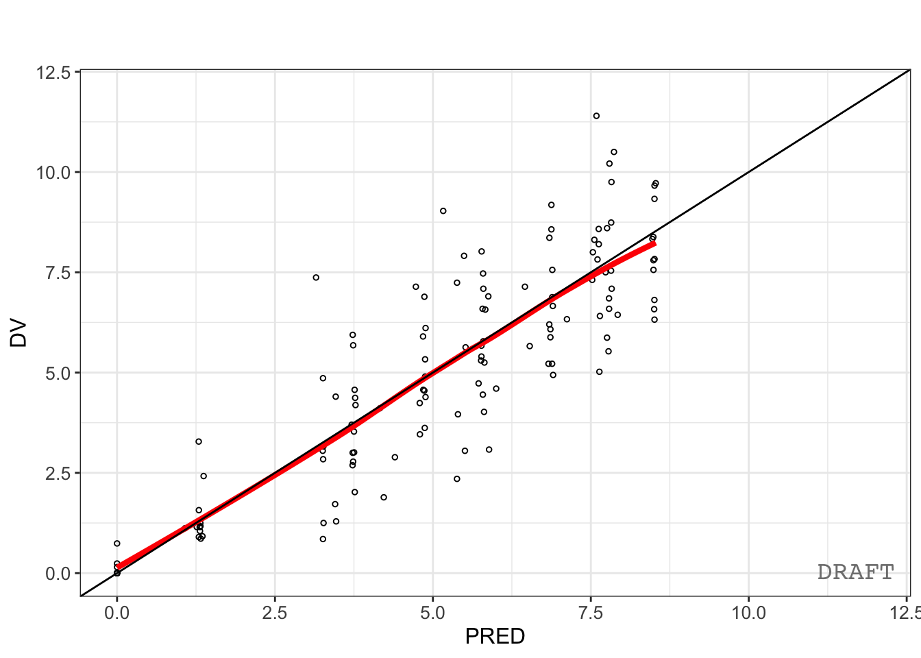
Residuals:
pmx_plot_cwres_pred(ctr)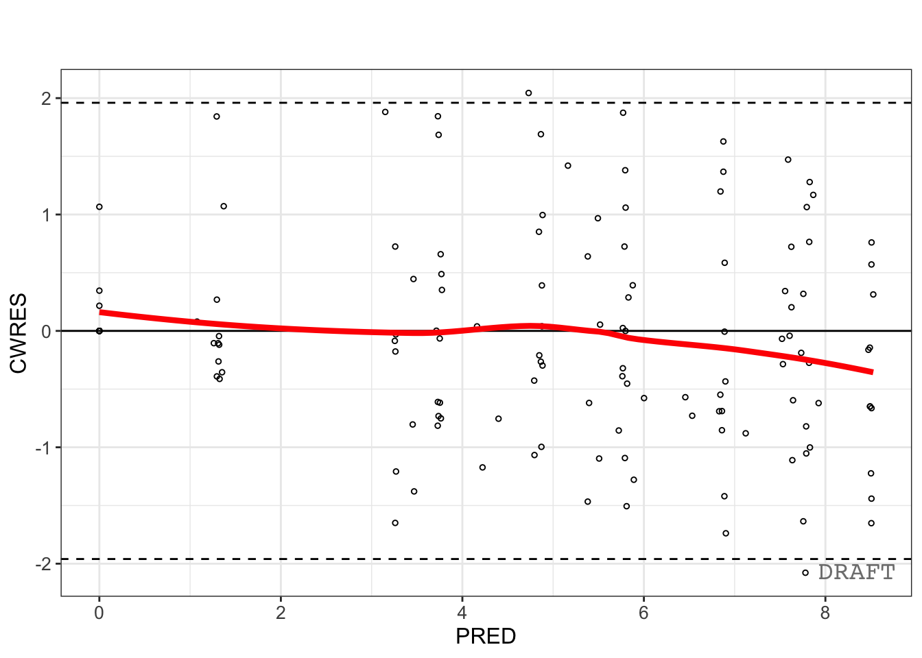
VPC:
vpcPlot(
  fit,
  n = 100,
  show = list(
    obs_dv = TRUE
  ),
  bins = "jenks",
  xlab = "Time",
  ylab = "Concentration"
)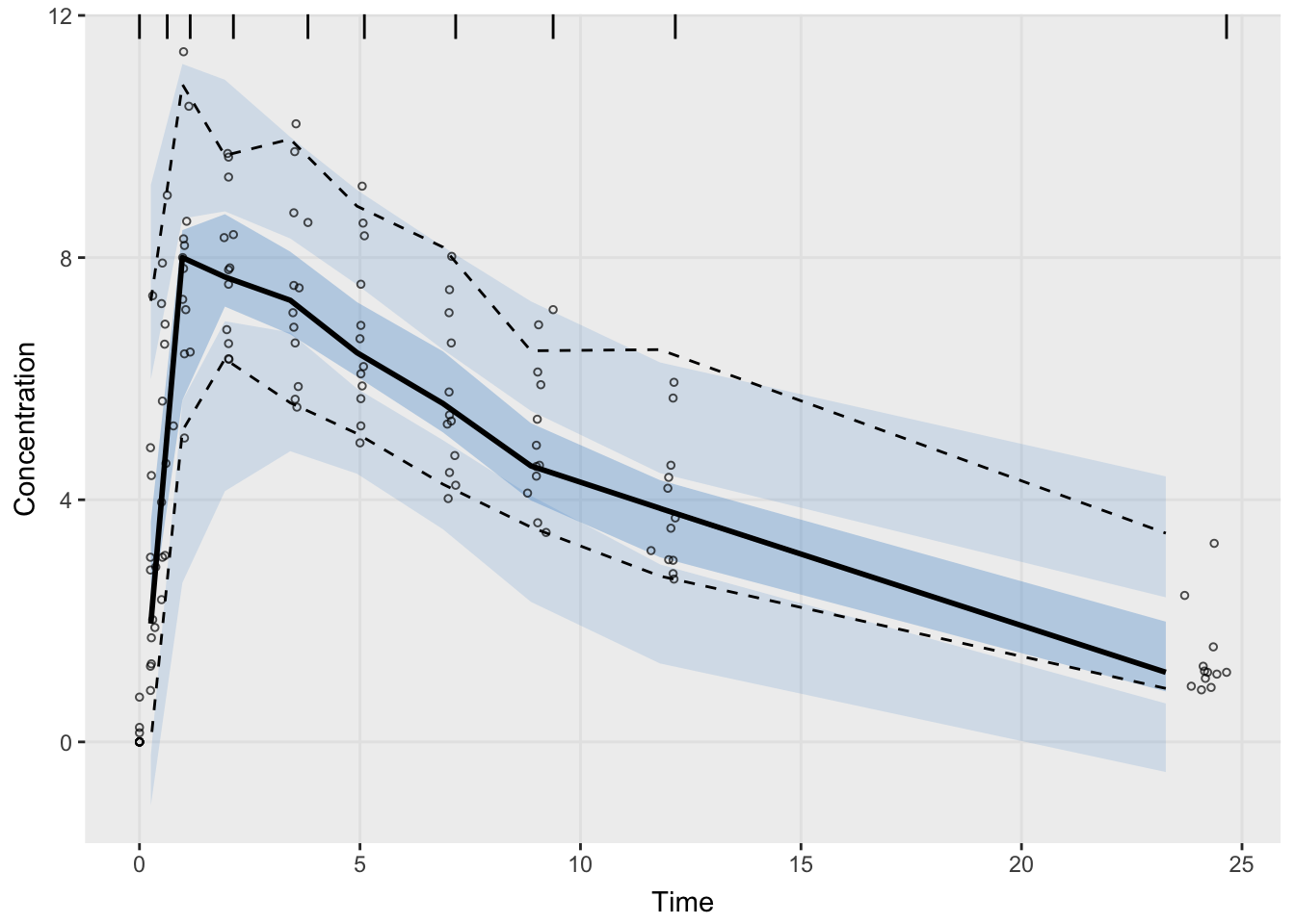
Interpretation:
No single diagnostic qualifies a model.
Ask:
Agreement

↓

Residual Behavior

↓

Variability

↓

Precision

↓

Adequate?
Qualification requires multiple lines of evidence.
Worked Example 4: Precision, Accuracy, and Qualification
These are related but different.
Precision ≠ Accuracy ≠ QualificationA model may be:
Precise but biasedor:
Less precise but usefulExamples:
Low %RSE + Poor Diagnostics = Not QualifiedHigher %RSE + Strong Diagnostics = Potentially UsefulInterpret estimates and diagnostics together.
Worked Example 5: Qualification Framework
Qualification integrates the full workflow.
Structure

↓

Variability

↓

Covariates

↓

Precision

↓

GOF

↓

Residuals

↓

VPC

↓

Decision Context

↓

Qualification
Qualification depends on intended use.
Examples:
| Intended Use | Qualification Standard |
|---|---|
| classroom learning | lower |
| descriptive analysis | moderate |
| simulation | higher |
| decision support | highest |
No single metric qualifies a model.
Strategies
- evaluate estimates and diagnostics together
- compare evidence across diagnostics
- think about intended use
- document limitations
Common Mistakes
- treating estimates as exact
- ignoring variability
- qualifying from one plot
- expecting perfect diagnostics
Practice Problems
What is parameter precision?
Why does low uncertainty not guarantee qualification?
Run:
print(fit)Identify:
- one estimate
- one uncertainty measure
Explain what each means.
- Run:
VarCorr(fit)What type of information does this provide?
- Suppose:
Low %RSE
Good GOF
Good Residuals
Poor VPC
Would the model be fully qualified? Explain.
TipStep-by-Step Solutions
Problem 1
Parameter precision describes how uncertain an estimate is.
Examples:
SE → uncertainty%RSE → relative uncertaintyPrecision answers:
How stable is the estimate?Problem 2
Low uncertainty alone does not guarantee adequacy.
A model may estimate parameters precisely while still producing:
- biased predictions
- poor residual behavior
- unrealistic variability
Diagnostics are still required.
Problem 3
Inspect:
print(fit)Examples:
Est. → estimated valueSE → uncertainty%RSE → relative uncertaintyInterpret these together.
Problem 4
VarCorr(fit) summarizes variability.
Examples include:
ETA variability → subject differencesand residual variability.
This helps determine whether variability estimates appear reasonable.
Problem 5
The model would not be fully qualified.
Interpretation:
Low %RSE → precise estimatesPoor VPC → poor variability reproductionQualification requires agreement across multiple diagnostics.
Summary
- uncertainty matters
- precision and accuracy differ
- qualification integrates diagnostics
- adequacy depends on purpose
TipQuick Tips
- Precision ≠ accuracy
- Qualification ≠ convergence
- Combine diagnostics
- Match evaluation to purpose