library(tidyverse)
library(nlmixr2data)

data("theo_sd", package = "nlmixr2data")Parameters and Profile Shape
Understand how structural PK parameters change concentration-time profiles.
Tip
Big picture: Structural parameters are not abstract numbers. Each parameter changes the concentration-time profile in a predictable way.
Learning Objectives
By the end of this lesson, you will be able to:
- Explain how
ka,CL, andVinfluence profile shape. - Predict how parameter changes affect concentration.
- Interpret parameter effects visually.
- Distinguish peak timing from elimination behavior.
- Build intuition before formal estimation.
Key Ideas
- Parameters determine profile shape.
- Structural interpretation should come before estimation.
- Different parameters influence different parts of the profile.
- Visualization builds modeling intuition.
Setup
Define the structural function.
one_comp_oral <- function(time, dose, ka, CL, V) {

  k <- CL / V

  dose * ka / (V * (ka - k)) * (exp(-k * time) - exp(-ka * time))
}
Why Parameter Interpretation Matters
Suppose two profiles differ.
Why?
Possible explanations:
- different absorption
- different clearance
- different volume
Understanding parameter effects makes later population models easier to interpret.
Worked Example 1: Simulate Parameter Scenarios
Create several structural scenarios.
time_grid <- seq(0, 24, length.out = 200)

scenarios <- tribble(
  ~scenario,     ~ka, ~CL, ~V,
  "Reference",     1,   3, 30,
  "Higher CL",     1,   6, 30,
  "Higher V",      1,   3, 60,
  "Higher ka",     2,   3, 30
)

profiles <-
scenarios %>%
  rowwise() %>%
  mutate(
    data = list(
      tibble(
        TIME = time_grid,
        CONC = one_comp_oral(time_grid, dose = 320, ka = ka, CL = CL, V = V)
      )
    )
  ) %>%
  unnest(data)
Plot the profiles.
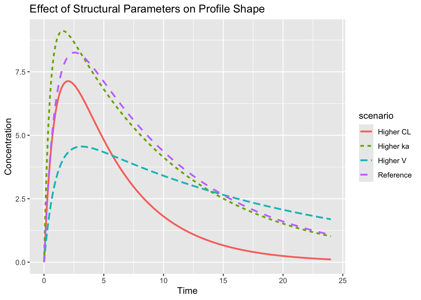
ggplot(
  profiles, aes(TIME, CONC, color = scenario, linetype = scenario)
) +
  geom_line(linewidth = 1) +
  labs(
    title = "Effect of Structural Parameters on Profile Shape",
    x = "Time",
    y = "Concentration"
  )
Worked Example 2: Higher Clearance
Higher clearance means drug leaves faster.
Conceptually:
Higher CL
↓
Higher k
↓
Faster elimination
↓
Lower concentrations
Interpretation:
- lower exposure
- steeper decline
- shorter half-life
Worked Example 3: Higher Volume
Higher volume changes concentration scaling.
Conceptually:
Higher V
↓
Lower concentration
↓
Broader profile
Interpretation:
- lower peak
- lower initial concentrations
- slower apparent decline
Remember:
\[ k=\frac{CL}{V} \]
Increasing V changes elimination behavior even when CL stays fixed.
Worked Example 4: Faster Absorption
Higher ka changes timing.
Conceptually:
Higher ka
↓
Drug enters faster
↓
Earlier peak
Interpretation:
- faster rise
- earlier peak
- elimination phase may remain similar
Absorption affects the beginning of the profile more than the terminal phase.
Worked Example 5: Compare Key Metrics
Extract simple summary metrics.
profile_summary <-
profiles %>%
  group_by(scenario) %>%
  summarise(cmax = max(CONC),
            tmax = TIME[which.max(CONC)],
            .groups = "drop")

profile_summary
# A tibble: 4 × 3
scenario cmax tmax
<chr> <dbl> <dbl>
1 Higher CL 7.13 2.05
2 Higher V 4.56 3.14
3 Higher ka 9.11 1.57
4 Reference 8.26 2.53Interpret:
Cmax→ peak concentrationTmax→ time of peak
Which Parameter Controls What?
| Parameter | Main Effect |
|---|---|
ka |
Peak timing |
CL |
Elimination speed |
V |
Concentration scaling |
Parameters interact, but this table is a useful starting approximation.
Connection to Population Models
Population models estimate these parameters across subjects.
Example:
Subject A
CL = 3

Subject B
CL = 5
Different parameters produce different profiles.
Population modeling learns both:
- typical values
- variability
Strategies
- Change one parameter at a time.
- Compare profiles visually.
- Build intuition before estimation.
- Connect parameters to biology.
Common Mistakes
- Memorizing equations without interpretation.
- Treating parameters independently.
- Ignoring profile shape.
Practice Problems
- What happens when
CLdoubles? - What happens when
Vdoubles? - What happens when
kaincreases? - Which parameter most strongly affects peak timing?
- Why do parameter effects overlap?
TipStep-by-Step Solutions
Problem 1: What happens when CL doubles?
If V stays fixed, doubling CL increases:
\[ k = \frac{CL}{V} \]
This makes elimination faster.
The concentration-time profile usually declines more steeply and exposure decreases.
Problem 2: What happens when V doubles?
A larger V means the same amount of drug is distributed into a larger apparent volume.
This usually lowers concentrations.
Because:
\[ k = \frac{CL}{V} \]
a larger V can also slow the apparent terminal decline if CL is unchanged.
Problem 3: What happens when ka increases?
Higher ka means faster absorption.
The profile usually rises more quickly and reaches peak concentration earlier.
The terminal elimination phase may be less affected if CL and V are unchanged.
Problem 4: Which parameter most strongly affects peak timing?
ka usually has the strongest direct effect on peak timing for an oral one-compartment model.
A faster absorption rate tends to shift Tmax earlier.
Problem 5: Why do parameter effects overlap?
PK parameters are connected.
For example, CL and V both influence elimination through:
\[ k = \frac{CL}{V} \]
So changing one parameter can affect more than one part of the profile.
Summary
- Structural parameters determine profile shape.
CL,V, andkahave interpretable effects.- Visualization builds intuition.
- Population models estimate these effects across subjects.
TipQuick Tips
CLremoves drug.Vspreads drug.kamoves drug into the system.- Compare profiles visually.