library(tidyverse)From Variability to Explanation
Connect covariate modeling back to the broader goals of population PK modeling.
Tip
Big picture: Population PK modeling is not only about estimating variability. It is about understanding why variability exists.
Learning Objectives
By the end of this lesson, you will be able to:
- connect variability and covariate modeling
- distinguish explained and unexplained variability
- understand how covariates relate to ETA
- interpret ETA-covariate relationships
- explain why covariates support decision making
Key Ideas
- variability is expected
- ETA describes unexplained variability
- covariates explain part of variability
- ETA usually remains
- explanation improves prediction and interpretation
Setup
Where We Started
Early population models often looked like:
\[ CL_i = TVCL \exp(\eta_i) \]
Interpretation:
Typical Clearance → Random Variability → Individual ClearanceQuestion:
Why do subjects differ?Random effects describe differences.
They do not explain them.
Worked Example 1: Variability Before Covariates
Before covariates:
Population Parameter → ETA → Individual ParameterConceptually:
\[ CL_i= TVCL \exp(\eta_i) \]
Interpretation:
Everything unexplained appears inside:
\[ \eta \]
Large or patterned ETA may indicate missing structure.
Worked Example 2: Add Covariates
Now extend the model:
\[ CL_i= TVCL \left( \frac{WT_i}{70} \right)^{\theta} \exp(\eta_i) \]
Interpretation:
Typical Value → Weight Effect → Remaining ETACovariates move some variability from:
unexplainedto:
explainedThis does not mean all variability disappears.
It means part of the variability now has an interpretable explanation.
Worked Example 3: ETA-Covariate Relationships
A common exploratory question is:
Does a covariate explain part of ETA?Create a simple simulated example.
set.seed(100)

eta_tbl_before <-
  tibble(
    WT = seq(40, 120, length.out = 100),
    ETA_CL = 0.02 * (WT - 70) + rnorm(100, 0, 0.2)
  )
Plot weight versus ETA for clearance before adding weight as a covariate.
ggplot(eta_tbl_before, aes(WT, ETA_CL)) +
  geom_point() +
  geom_smooth(se = FALSE) +
  labs(
    title = "Weight vs ETA(CL) Before Adding Weight",
    x = "Weight",
    y = "ETA(CL)"
  )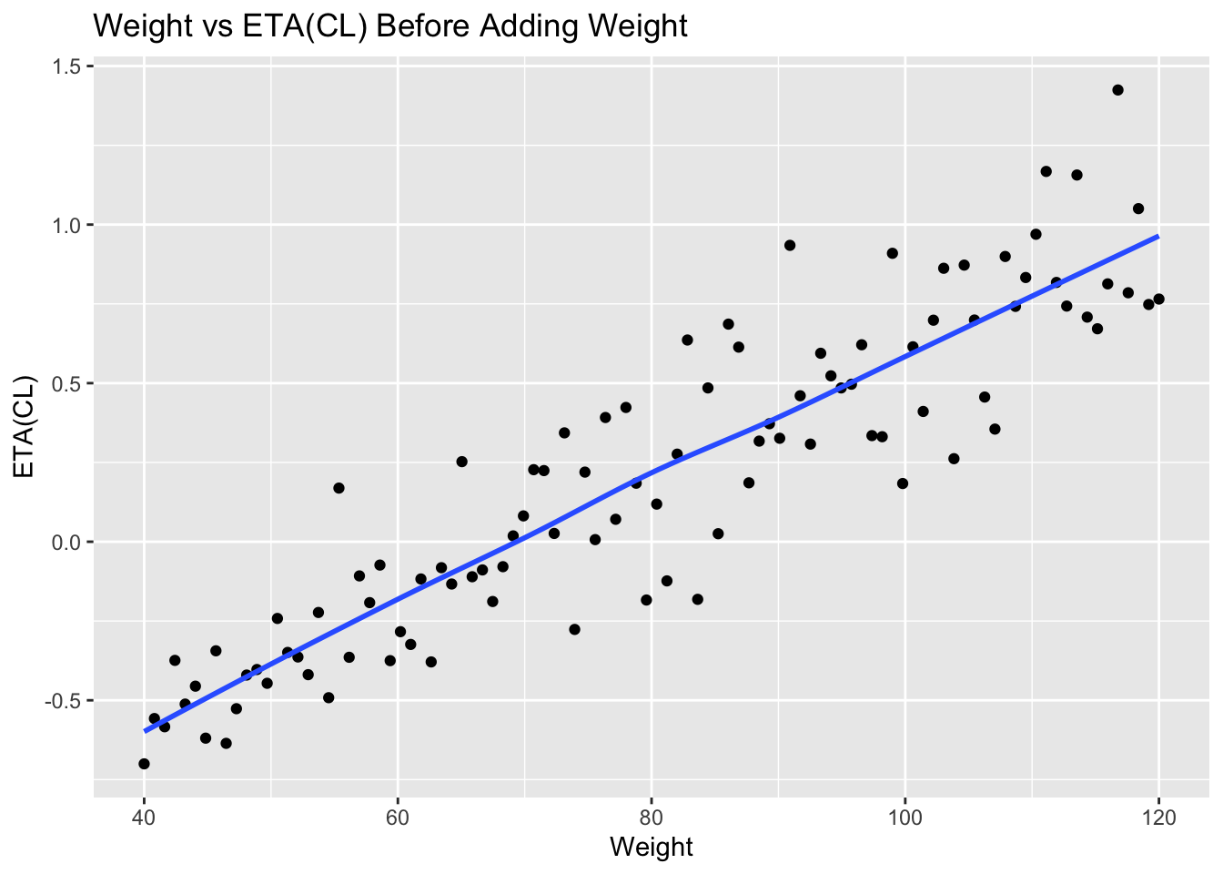
Interpretation:
A visible trend may suggest that weight explains part of the remaining variability in clearance.
Now simulate a situation where the weight trend has been accounted for.
set.seed(101)

eta_tbl_after <-
  tibble(
    WT = seq(40, 120, length.out = 100),
    ETA_CL = rnorm(100, 0, 0.2)
  )
Plot weight versus ETA again.
ggplot(eta_tbl_after, aes(WT, ETA_CL)) +
  geom_point() +
  geom_smooth(se = FALSE) +
  labs(
    title = "Weight vs ETA(CL) After Adding Weight",
    x = "Weight",
    y = "ETA(CL)"
  )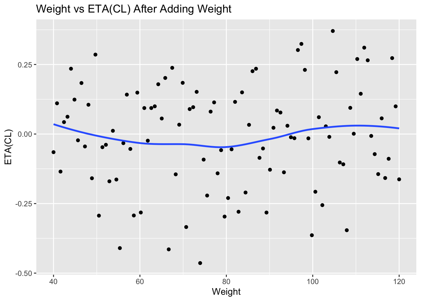
Interpretation:
After a useful covariate is added, the relationship between the covariate and ETA should be reduced.
The goal is not to remove ETA completely.
The goal is to move systematic patterns out of ETA and into the fixed-effects portion of the model.
Worked Example 4: Explained vs Unexplained Variability
Conceptually:
Before:
Total Variability = ETAAfter:
Total Variability = Covariate Effect + Remaining ETAInterpretation:
Covariates usually reduce unexplained variability.
They rarely eliminate it.
Some variability remains because not all differences between individuals are measured, modeled, or biologically understood.
Worked Example 5: Why Explanation Matters
Two models may predict similarly.
But one may explain more.
Model A:
Prediction ✓

Interpretation ✗
Model B:
Prediction ✓

Interpretation ✓
Population modeling values both prediction and explanation.
Explanation supports biological understanding.
Worked Example 6: Population Thinking
Population modeling does not attempt to perfectly describe every individual.
Instead:
Population → Covariates → Subgroups → IndividualsInterpretation:
We improve predictions by understanding systematic differences.
Covariates help describe how typical parameter values change across the population.
Covariates Support Decisions
Examples:
- identify dose adjustments
- understand exposure differences
- characterize patient populations
- support study design
- support individualized medicine
Interpretation matters beyond estimation.
Covariates Are Not Always Needed
Questions:
- biologically plausible?
- clinically meaningful?
- measurable?
- reproducible?
A more complex model is not automatically better.
A useful covariate should improve understanding, prediction, or decision making.
Covariates Connect Modules
What we have learned:
Data → Structural Model → Population Model → Variability → CovariatesUpcoming modules will ask:
Did the model improve?That leads toward:
- diagnostics
- model qualification
- simulation
Looking Ahead
We now understand:
Describe Variability → Explain VariabilityNext we move toward evaluating whether the explanation improved the model.
Strategies
- look for patterns in ETA
- explain before optimizing
- interpret before concluding
- prioritize biology
- remember that ETA usually remains
Common Mistakes
- assuming ETA should disappear
- treating every ETA-covariate trend as causal
- reporting only coefficients
- assuming complexity means quality
- ignoring biological plausibility
Practice Problems
What is the difference between explained and unexplained variability?
Why do covariates usually not eliminate ETA?
What might a trend between ETA(CL) and weight suggest?
Why is explanation valuable?
Why are complex models not always better?
TipStep-by-Step Solutions
Problem 1
Explained variability comes from systematic differences included in the model.
Unexplained variability remains in ETA.
Problem 2
Not all variability is measurable, modeled, or biologically understood.
Problem 3
It may suggest that weight explains part of the remaining variability in clearance.
Problem 4
Explanation improves understanding, supports prediction, and helps inform decisions.
Problem 5
Additional complexity may reduce interpretability, add instability, or describe patterns that are not reproducible.
Summary
- ETA describes unexplained variability
- covariates explain part of variability
- ETA-covariate plots can suggest missing covariate structure
- useful covariates reduce systematic patterns in ETA
- ETA usually remains
- explanation supports decisions
TipQuick Tips
- Look at ETA patterns
- Explain variability
- Keep ETA
- Biology first
- Interpretation matters