library(tidyverse)
library(nlmixr2)
library(nlmixr2data)

data("theo_sd", package = "nlmixr2data")Running FOCEi Estimation
Fit the first population PK model using nlmixr2 and understand the estimation workflow.
Tip
Big picture: Estimation combines a model with observed data and searches for parameter values that explain the observations reasonably well.
Learning Objectives
By the end of this lesson, you will be able to:
- Run the first
nlmixr2estimation. - Understand FOCEi conceptually.
- Explain why initial values matter.
- Distinguish model definition from model estimation.
- Recognize that estimation returns a fit object.
Key Ideas
- Estimation combines a model with observed data.
- FOCEi searches for parameter values that improve agreement.
- Initial values guide optimization but are not final estimates.
- Estimation returns parameter estimates and model output.
Setup
Why Estimation Exists
Until now we selected parameters manually.
Example:
CL = 3
V = 30
ka = 1
But real modeling asks:
Which parameter values best explain the observations?
Estimation attempts to answer that question.
Conceptually:
Observed Data
↓
Model Predictions
↓
Compare
↓
Update Parameters
↓
Repeat
This repeated search is called optimization.
The goal is not to perfectly match every observation.
The goal is to find parameter values that explain the data reasonably well.
Worked Example 1: Define the First Population PK Model
one_comp_model <- function(){

  ini({

    tka <- log(1)
    tcl <- log(3)
    tv  <- log(30)

    eta.ka ~ 0.1
    eta.cl ~ 0.1
    eta.v  ~ 0.1

    add.err <- 0.1

  })

  model({

    ka <- exp(tka + eta.ka)
    cl <- exp(tcl + eta.cl)
    v  <- exp(tv + eta.v)

    linCmt() ~ add(add.err)

  })

}
Notice what changed compared with the structural simulations.
The model now includes:
Typical Values
↓
Subject Variability
↓
Residual Error
For now, focus on the estimation workflow.
The next module explains variability and residual error in more detail.
Worked Example 2: Run FOCEi
Estimate the model.
fit <-
  nlmixr2(
    one_comp_model,
    theo_sd,
    est = "focei",
    control = list(
      print = 0
    )
  )
This step combines:
Model
+
Data
+
Estimation
↓
Fit Object
Internally, estimation repeatedly:
Generate Predictions
↓
Compare to Data
↓
Adjust Parameters
↓
Repeat
This repeated search is optimization.
The exact mathematics are less important here than the overall workflow.
Note
control = list(
  print = 0
)
reduces estimation output so the lesson focuses on model interpretation rather than optimization logs.
Increase printing later if debugging convergence.
NoteOptional: How Optimization Converges
Until now, estimation has behaved like a black box.
Optimization updates parameter estimates repeatedly until the fit stabilizes.
Generate diagnostic plots.
pl <- plot(fit)Display the optimization trace.
pl$traceplot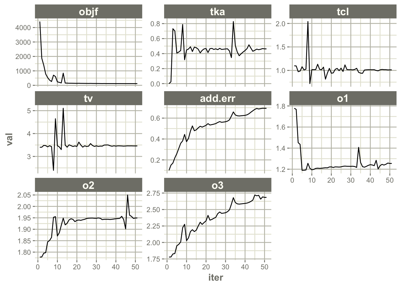
Interpretation:
The plot shows how parameter estimates evolve during optimization.
Look for:
- noticeable movement early
- smaller updates later
- stabilization toward the end
Conceptually:
Initial Values

↓

Parameter Updates

↓

Convergence
Question:
Did estimation appear to settle?Do not expect perfectly flat lines.
Small movement near convergence can be normal.
This plot helps visualize optimization behavior.
Routine model evaluation later focuses on diagnostics rather than optimization traces.
What Is Maximum Likelihood?
Most population estimation methods are based on the idea of likelihood.
Conceptually:
Model Parameters

↓

Generate Predictions

↓

Compare with Observations

↓

Score Agreement
Likelihood asks:
If these parameter values were true, how likely would the observed data be?
Estimation searches for parameter values that improve that agreement.
Conceptually:
Higher Likelihood

↓

Better Agreement
Internally, FOCEi optimizes an objective function value (OFV), which is related to likelihood:
\[ OFV = -2\log L \]
Better agreement between observations and model predictions generally leads to a lower OFV.
Conceptually:
Higher Likelihood

↓

Lower OFV

↓

Better Agreement
Most pharmacometric software reports OFV rather than likelihood directly.
FOCEi is one method used to approximate this process efficiently.
For now:
do not think of likelihood as probability of the model being correct.
Think of it as a scoring system that rewards agreement between:
Observed Data

↓

Predicted Data
Later courses revisit likelihood in more mathematical detail.
Worked Example 3: Inspect the Model Representation
View the fitted model.
fit\[\begin{align*} {ka} & = \exp\left({tka}+{eta.ka}\right) \\ {cl} & = \exp\left({tcl}+{eta.cl}\right) \\ {v} & = \exp\left({tv}+{eta.v}\right) \\ linCmt() & \sim add({add.err}) \end{align*}\]
The rendered output displays the fitted model structure.
Notice how the model is represented as equations:
Typical Parameters
↓
Subject Variability
↓
Prediction
This view is useful because it reminds us what model was estimated.
Focus on recognizing:
- parameter relationships
- variability structure
- observation model
Detailed fit output is covered in the next lesson.
Worked Example 4: Extract Fixed Effects
Extract fixed-effect estimates.
coef(fit)$fixed %>%
enframe(
  name = "parameter",
  value = "estimate"
)
# A tibble: 4 × 2
parameter estimate
<chr> <dbl>
1 tka 0.463
2 tcl 1.01
3 tv 3.46
4 add.err 0.694Back-transform estimates.
coef(fit)$fixed %>%
exp() %>%
enframe(
  name = "parameter",
  value = "estimate_original_scale"
)
# A tibble: 4 × 2
parameter estimate_original_scale
<chr> <dbl>
1 tka 1.59
2 tcl 2.75
3 tv 31.8
4 add.err 2.00Interpretation:
tka→ typical absorptiontcl→ typical clearancetv→ typical volume
These are estimated values.
They are no longer manually selected guesses.
Worked Example 5: What Is FOCEi Doing?
FOCEi stands for:
First-Order Conditional Estimation with Interaction
You do not need to memorize the acronym.
For now, remember:
Model
+
Data
↓
Optimization
↓
Parameter Estimates
FOCEi is one estimation method.
Other approaches include:
- SAEM
- Bayesian estimation
- simulation-based estimation
Later courses can discuss estimation algorithms in greater detail.
Why Are There Multiple Estimation Methods?
Different models create different estimation challenges.
Examples:
| Method | Typical Use |
|---|---|
| FOCEi | standard population PK models |
| SAEM | difficult models or sparse data |
| Bayesian methods | prior information and full uncertainty |
| Simulation-based methods | specialized workflows |
Conceptually:
Simple Model
↓

FOCEi

Complex Model
↓

Alternative Methods
For this course:
FOCEi = default starting pointbecause it is:
- widely used
- fast
- interpretable
- well suited for many PK models
Reading Estimation Output
After estimation, ask:
- Did estimation finish?
- Are estimates reasonable?
- Did optimization converge?
- Did initial values appear adequate?
Do not judge diagnostics yet.
Diagnostics evaluate model adequacy later.
Strategies
- Start simple.
- Check whether the model runs.
- Keep initial estimates biologically reasonable.
- Interpret large features first.
Common Mistakes
- Treating estimates as truth.
- Ignoring convergence.
- Overinterpreting early results.
- Assuming one estimation method is always best.
Practice Problems
Why is estimation needed?
What does FOCEi do conceptually?
What information is stored in
fit?Run:
fitWhat does this output show?
Then run:
coef(fit)$fixedWhy is this easier for numerical interpretation?
- Modify one initial estimate.
Change:
tv <- log(30)to:
tv <- log(20)Refit the model.
Did estimation still converge?
If not:
- what might have changed?
- why can starting values matter?
TipStep-by-Step Solutions
Problem 1
Estimation learns parameters from observed data.
Instead of choosing:
CL = 3the algorithm searches for values that explain the data.
Conceptually:
Data
+
Model
↓
Estimated Parameters
Problem 2
FOCEi repeatedly:
Generate Predictions
↓
Compare to Data
↓
Update Parameters
↓
Repeat
until optimization stabilizes.
It is a search procedure for parameter values.
Problem 3
fit stores model output.
Examples include:
- parameter estimates
- model equations
- predictions
- residual quantities
- estimation metadata
The fit object becomes the central object for later interpretation.
Problem 4
Running:
fitshows the fitted model representation.
This is useful for understanding:
- equations
- parameter relationships
- model structure
For numerical interpretation, use:
coef(fit)$fixedThis extracts fixed-effect estimates directly.
It is easier than reading values from the rendered model object.
Problem 5
Changing initial values changes where optimization begins.
If the new initial value is still reasonable, estimation may converge to similar estimates.
If the initial value is poor, estimation may:
- take longer
- converge to a different solution
- fail to converge
Initial values matter because optimization is an iterative search.
Summary
- Estimation combines models and data.
- FOCEi is an optimization-based estimation method.
- Initial values guide the search.
nlmixr2returns a fit object.- Detailed fit interpretation comes next.
TipQuick Tips
- Start simple.
- Initial values matter.
- Fit first, diagnose later.
- Interpret before optimizing.