library(tidyverse)Direct Effect Models
Build the first PK/PD models by connecting concentration directly to response.
Tip
Big picture: Direct effect models assume response changes immediately as concentration changes.
Learning Objectives
By the end of this lesson, you will be able to:
- explain direct response models
- distinguish linear and Emax relationships
- interpret Emax and EC50
- simulate exposure–response relationships
- recognize saturation
Key Ideas
- concentration drives effect
- response may increase nonlinearly
- saturation is common
- PD parameters have biological interpretation
Setup
This lesson uses simulated examples.
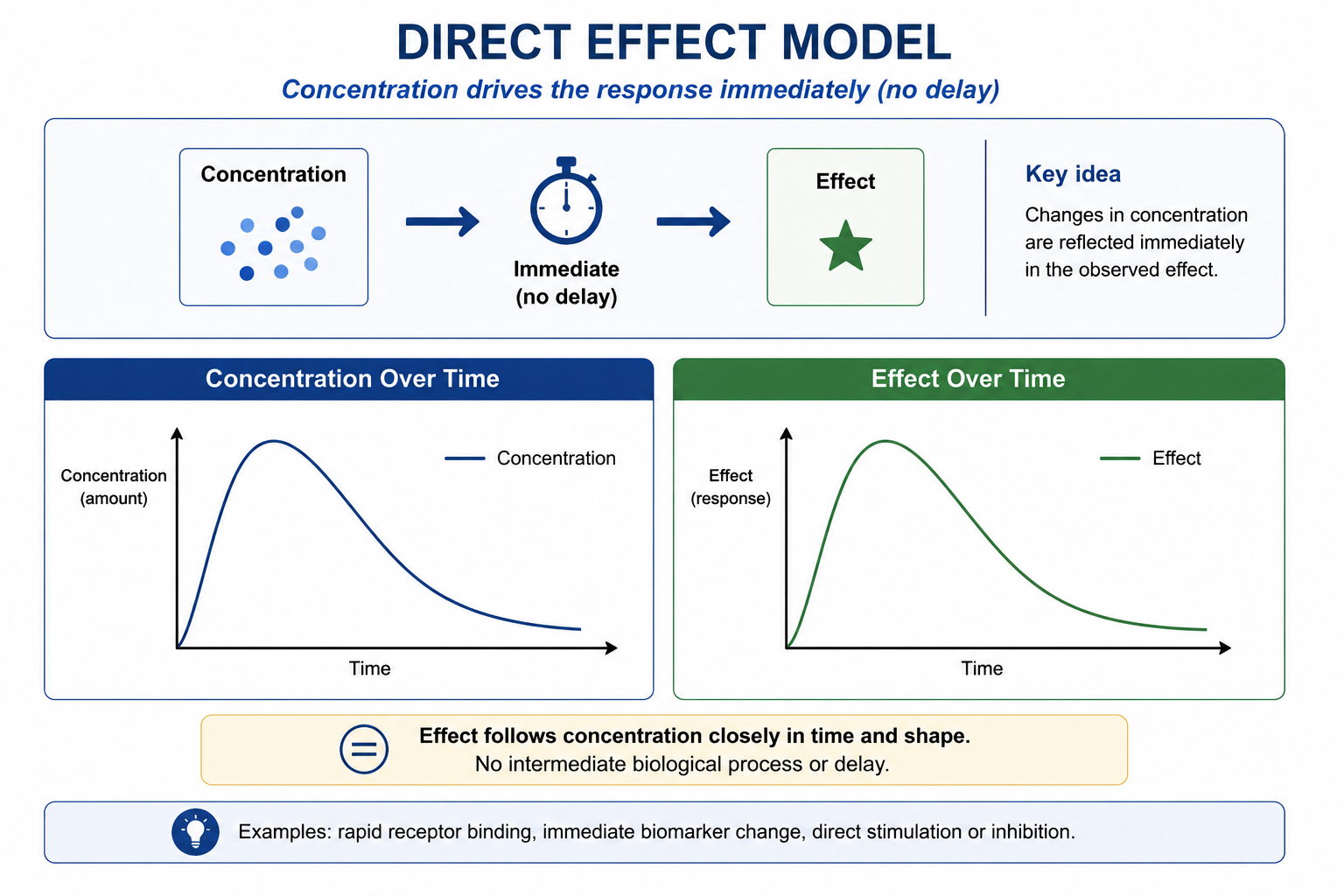
What Is a Direct Effect Model?
Direct effect assumes:
Concentration → ResponseResponse changes immediately as concentration changes.
There is no delay.
Examples:
- rapid receptor binding
- immediate biomarker change
Worked Example 1: Linear Effect Model
A simple possibility is a linear relationship.
\[ E = E_0 + S C \]
Interpretation:
| Parameter | Meaning |
|---|---|
| \(E_0\) | baseline effect |
| \(S\) | sensitivity |
| \(C\) | concentration |
Question:
Does each increase in concentration produce the same effect increase?Simulate.
conc <-
  tibble(
    C = seq(0, 100, by = 1)
  )

lin_effect <-
  conc %>%
  mutate(
    E = 20 + 0.8 * C
  )

ggplot(
  lin_effect,
  aes(C, E)
) +
geom_line() +
labs(
  title = "Linear Effect",
  x = "Concentration",
  y = "Effect"
)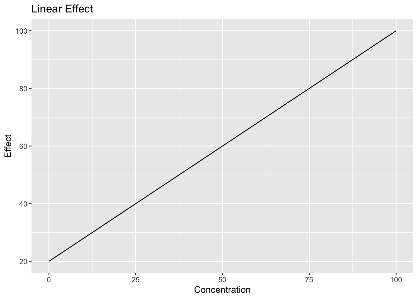
Interpretation:
Effect increases proportionally.
Worked Example 2: Why Linear Models Fail
Suppose concentration continues increasing.
Question:
Should response increase forever?Usually not.
Many systems saturate.
Conceptually:
More Exposure
↓
Smaller Additional Effect
This motivates Emax.
Worked Example 3: Emax Model
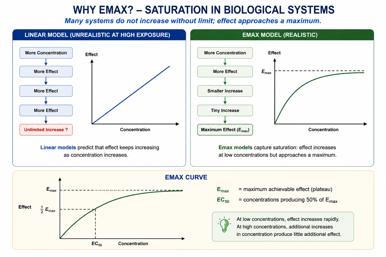
Introduce saturation.
\[ E = E_0 + \frac{E_{max} C}{EC_{50} + C} \]
Interpretation:
| Parameter | Meaning |
|---|---|
| \(E_0\) | baseline |
| \(E_{max}\) | maximum effect |
| \(EC_{50}\) | concentration producing half-maximal effect |
Question:
How much exposure is needed to generate effect?Simulate.
emax_effect <-
  conc %>%
  mutate(
    E = 20 + (100 * C / (10 + C))
  )

ggplot(
  emax_effect,
  aes(C, E)
) +
geom_line() +
labs(
  title = "Emax Relationship",
  x = "Concentration",
  y = "Effect"
)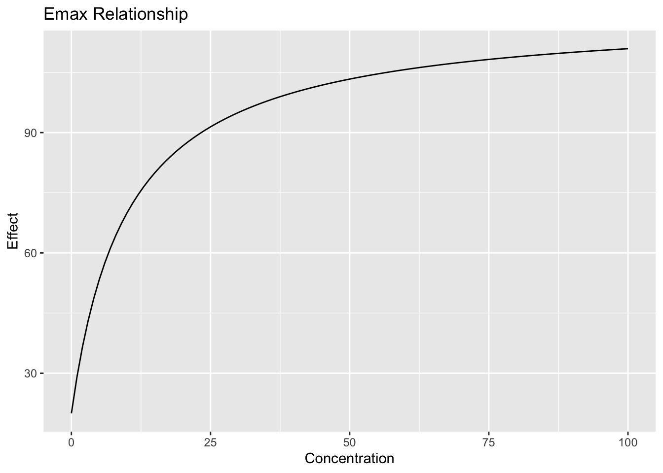
Interpretation:
Effect rises rapidly.
Then approaches a maximum.
Extension: Sigmoid Emax (Hill) Models
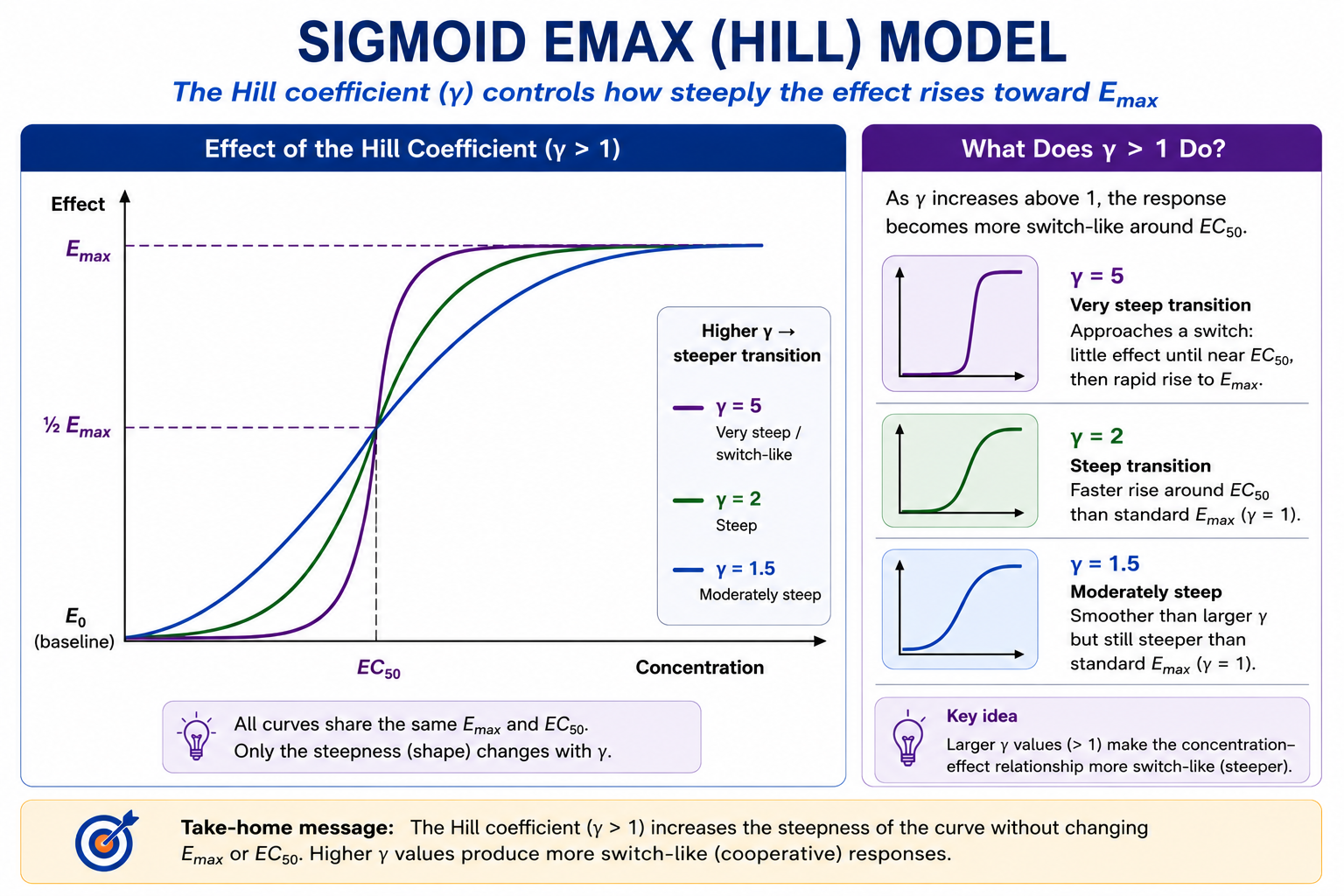
The Emax model assumes a smooth transition toward maximum effect.
Sometimes response changes more abruptly.
A common extension is the sigmoid Emax (Hill) model.
\[ E = E_0 + \frac{ E_{max} C^{\gamma} }{ EC_{50}^{\gamma} + C^{\gamma} } \]
Interpretation:
| Parameter | Meaning |
|---|---|
| \(E_0\) | baseline |
| \(E_{max}\) | maximum effect |
| \(EC_{50}\) | half-maximal concentration |
| \(\gamma\) | Hill coefficient |
The Hill coefficient controls curve shape.
Higher γ → steeper transition

Lower γ → smoother transition
Question:
Does response switch gradually or sharply?Examples:
- receptor cooperativity
- steep concentration–effect relationships
Simulate different Hill coefficients.
hill_tbl <-
  crossing(
    C = seq(0, 100, by = 0.1),
    gamma = c(0.5, 1, 5)
  ) %>%
  mutate(
    E =
      100 *
      C^gamma /
      (10^gamma + C^gamma)
  )

ggplot(
  hill_tbl,
  aes(
    C,
    E,
    linetype = factor(gamma)
  )
) +
  geom_line(linewidth = 1) +
  labs(
    title = "Effect of the Hill Coefficient",
    x = "Concentration",
    y = "Effect",
    linetype = expression(gamma)
  )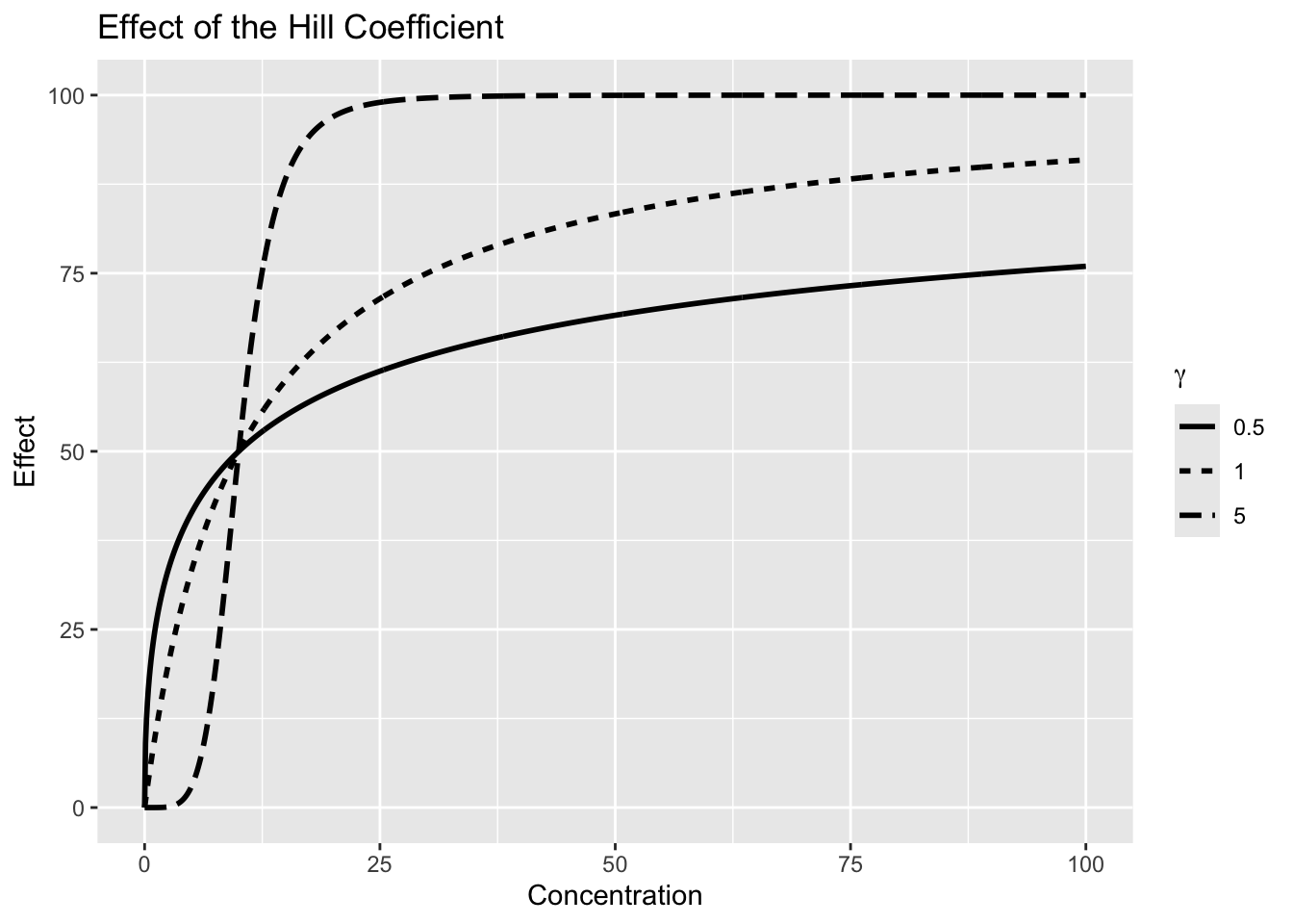
Interpretation:
- \(\gamma = 1\) produces the standard Emax model
- larger values of \(\gamma\) produce steeper, more switch-like behavior
- smaller values of \(\gamma\) produce more gradual transitions
For simplicity, this course primarily uses the standard Emax model.
Worked Example 4: Understanding EC50
EC50 controls horizontal position.
Example:
Lower EC50 → less concentration needed

Higher EC50 → more concentration needed
EC50 is often interpreted as a measure of potency.
Conceptually:
Lower EC50 → higher potency

Higher EC50 → lower potency
A more potent drug achieves the same effect at a lower concentration.
Simulate.
ec_tbl <-
  crossing(
    C = seq(0, 100, by = 1),
    EC50 = c(5, 10, 20)
  ) %>%
  mutate(
    E = 100 * C / (EC50 + C)
  )

ggplot(
  ec_tbl,
  aes(C, E, group = EC50)
) +
geom_line(
  aes(
    linetype =
      factor(EC50)
  )
) +
labs(
  title = "Effect of EC50",
  x = "Concentration",
  y = "Effect",
  linetype = "EC50"
)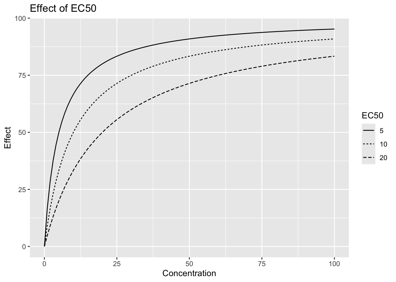
Interpretation:
Smaller EC50 shifts the concentration–effect relationship to the left.
At any given effect level, less concentration is needed.
This is often described as higher potency.
Worked Example 5: Direct Effect Thinking
Direct effect models answer:
Exposure

↓

Immediate Response
Questions become:
- how large?
- how sensitive?
- when does saturation occur?
Direct models are useful.
But many responses are delayed.
That motivates the next lesson.
Strategies
- visualize curves
- interpret parameters biologically
- compare shapes
Common Mistakes
- assuming larger concentration always helps
- treating EC50 as efficacy
- ignoring limits
Practice Problems
What assumption defines direct effect?
What does Emax represent?
What does EC50 represent?
Why can linear models fail?
What happens when EC50 decreases?
TipStep-by-Step Solutions
Problem 1
Concentration → ResponseProblem 2
Maximum achievable effect.
Problem 3
Half-maximal concentration.
Problem 4
Response often saturates.
Problem 5
Response shifts left.
Summary
- direct models connect exposure and response
- Emax introduces saturation
- EC50 controls sensitivity
- parameters explain biology
TipQuick Tips
- Direct ≠ delayed
- EC50 ≠ efficacy
- Saturation matters