library(tidyverse)
library(nlmixr2data)

data("theo_sd", package = "nlmixr2data")Simulating Structural PK Profiles in R
Use structural PK equations to generate and explore concentration-time profiles.
Tip
Big picture: Simulation allows us to understand how models behave before fitting them to data.
Learning Objectives
By the end of this lesson, you will be able to:
- Simulate structural PK profiles.
- Build concentration-time curves from parameter values.
- Compare multiple simulation scenarios.
- Understand sensitivity to parameter changes.
- Connect simulation to later population modeling.
Key Ideas
- Simulation generates predictions from assumptions.
- Structural simulation helps build intuition.
- Simulation and estimation are closely related.
- Models should be explored before fitting.
Setup
Define the structural model.
one_comp_oral <- function(time, dose, ka, CL, V) {

  k <- CL / V

  dose * ka / (V * (ka - k)) * (exp(-k * time) - exp(-ka * time))
}
This function manually implements the analytic structural solution.
Later, nlmixr2 and rxode2 will automate this process and allow more flexible model definitions.
Why Simulate?
Simulation lets us answer questions such as:
- What profile do these parameters produce?
- What happens if clearance changes?
- What happens if the dose changes?
- What happens before collecting data?
Simulation helps us understand the model before estimation.
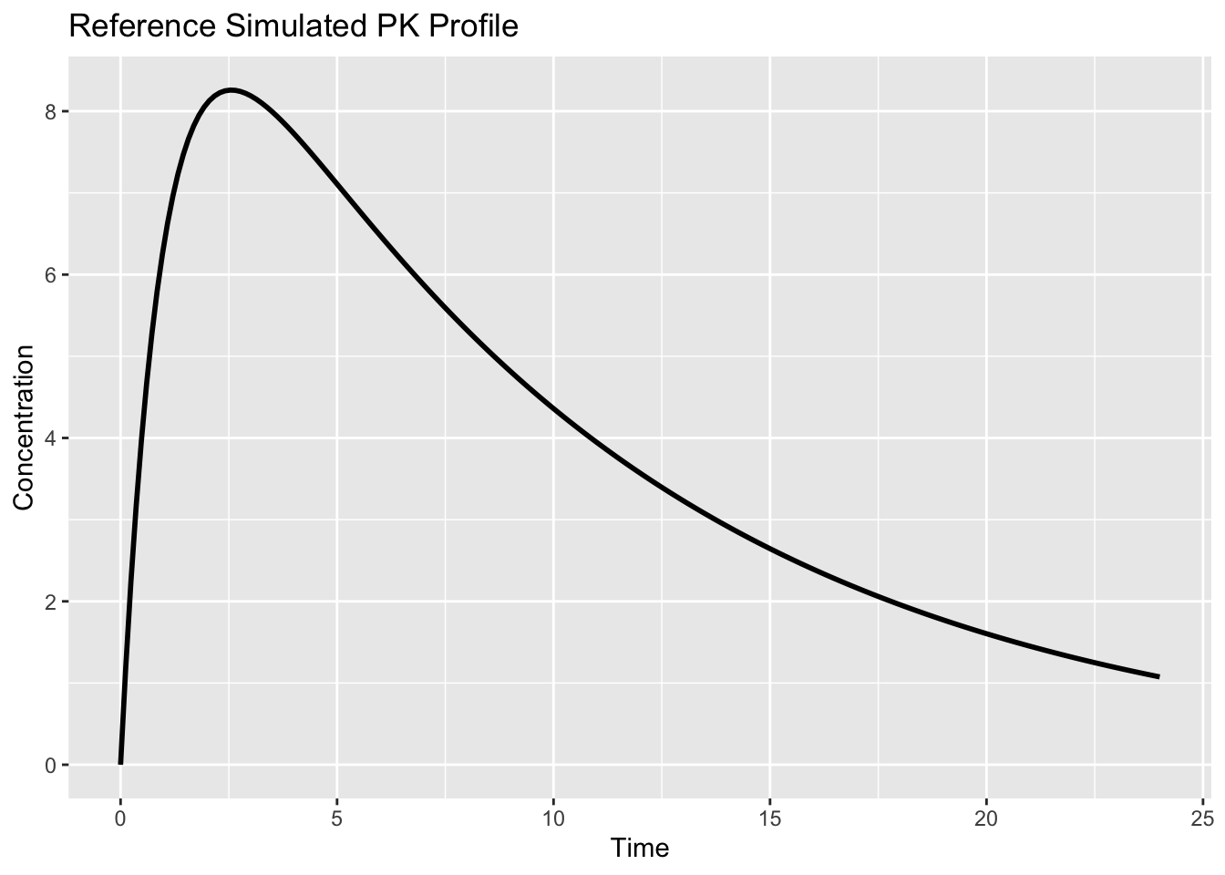
Worked Example 1: Simulate a Reference Profile
Create a time grid.
time_grid <- seq(0, 24, length.out = 200)Generate concentrations.
sim_ref <-
tibble(
  TIME = time_grid,
  CONC =
    one_comp_oral(
      time = time_grid,
      dose = 320,
      ka = 1,
      CL = 3,
      V = 30
    )
)
Visualize.
ggplot(sim_ref, aes(TIME, CONC)) +
  geom_line(linewidth = 1) +
  labs(
    title = "Reference Simulated PK Profile",
    x = "Time",
    y = "Concentration"
  )
Worked Example 2: Simulate Multiple Doses
Keep parameters fixed and vary dose.
dose_grid <-
c(160, 320, 640)

profiles <-
  crossing(
    TIME = time_grid,
    DOSE = dose_grid
  ) %>%
  mutate(
    CONC =
      one_comp_oral(
        TIME,
        dose = DOSE,
        ka = 1,
        CL = 3,
        V = 30
      )
  )
Plot.
ggplot(
  profiles,
  aes(
    TIME,
    CONC,
    color = factor(DOSE)
  )
) +
geom_line(
  linewidth = 1) +
  labs(
    title = "Effect of Dose on Profile Shape",
    x = "Time",
    y = "Concentration",
    color = "Dose"
  )
Interpretation:
- higher dose increases concentration
- profile shape remains similar
- this reflects linear kinetics
Worked Example 3: Simulate Different Subjects
Now vary parameters.
subjects <-
tribble(
~subject, ~ka, ~CL, ~V,
"A", 1.0, 3, 30,
"B", 1.0, 5, 30,
"C", 2.0, 3, 40
)

subject_profiles <-
  subjects %>%
  rowwise() %>%
  mutate(data = list(
    tibble(
      TIME = time_grid,
      CONC = one_comp_oral(
      time_grid,
      320,
      ka,
      CL,
      V
      )
    )
  )
) %>%
  unnest(data)
Plot.
ggplot(
  subject_profiles,
  aes(
    TIME,
    CONC,
    color = subject
  )
) +
  geom_line(
    linewidth = 1
  ) +
  labs(
    title = "Different Parameters Produce Different Profiles",
    x = "Time",
    y = "Concentration"
  )
Interpretation:
Different structural parameters generate different profiles.
Population models learn these differences.
Worked Example 4: Compare Simulation and Observation
Overlay simulation and observed data.
obs <-
theo_sd %>%
filter(
  EVID == 0
)

ggplot() +
  geom_point(data = obs, aes(TIME, DV), alpha = 0.25) +
  geom_line(data = sim_ref, aes(TIME, CONC), linewidth = 1) +
  labs(
    title = "Observed Data vs Structural Simulation",
    x = "Time",
    y = "Concentration"
    )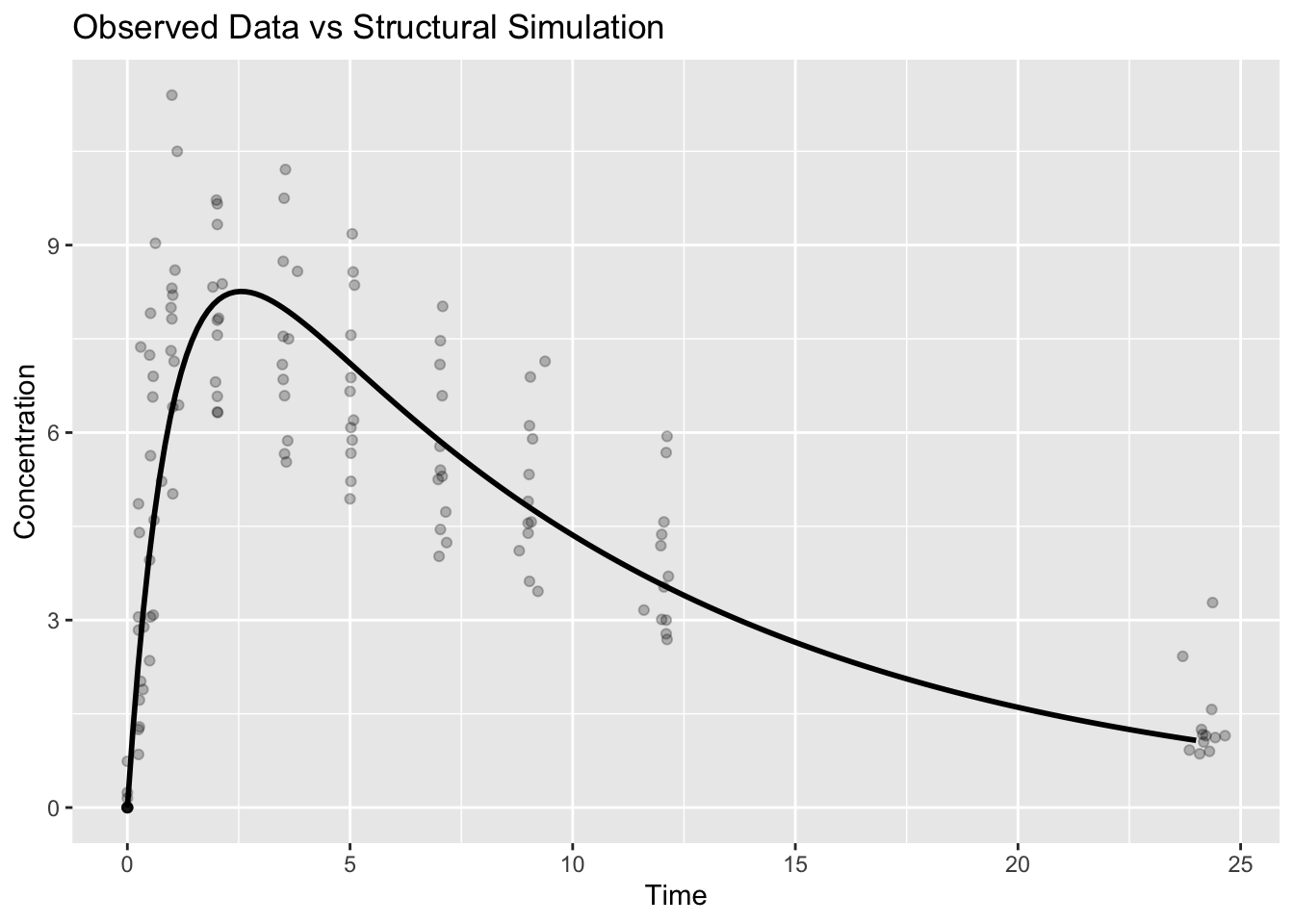
Interpretation:
A structural model does not need to pass through every point.
Its purpose is to represent the expected behavior.
Worked Example 5: Simulation Workflow
Conceptually:
Parameter Values
↓
Structural Equation
↓
Predicted Concentration
↓
Visualization
↓
Interpretation
This same idea later becomes:
Initial Estimates
↓
Population Model
↓
Estimation
↓
Diagnostics
Strategies
- Simulate before estimating.
- Change one parameter at a time.
- Compare scenarios visually.
Common Mistakes
- Treating simulation as validation.
- Forgetting assumptions.
- Ignoring biological interpretation.
Practice Problems
- Double the dose.
- Increase clearance.
- Decrease volume.
- Create a new simulated subject.
- Compare simulation to observations.
TipStep-by-Step Solutions
Problem 1: Double the dose.
Doubling the dose should approximately double the concentration values under linear PK.
The overall shape should remain similar because ka, CL, and V are unchanged.
This is an example of dose-proportional behavior.
Problem 2: Increase clearance.
Increasing CL makes elimination faster when V stays fixed.
The simulated profile should decline more rapidly and have lower exposure.
This is because CL increases the elimination rate constant:
\[ k = \frac{CL}{V} \]
Problem 3: Decrease volume.
A smaller V usually increases concentrations because the same amount of drug is distributed into a smaller apparent space.
It may also increase k if CL is unchanged.
So both concentration scale and terminal decline may change.
Problem 4: Create a new simulated subject.
A new simulated subject can be represented by choosing a new set of parameter values.
For example, one subject might have:
new_subject <- tibble(
  subject = "D",
  ka = 1.2,
  CL = 4,
  V = 35
)
The goal is not to claim this is a real subject.
The goal is to see how parameter differences generate different profiles.
Problem 5: Compare simulation to observations.
The simulated curve represents expected behavior from chosen parameters.
Observed data include variability and residual error.
So the curve should capture the general trend, but it should not be expected to pass through every point.
Summary
- Structural models generate predictions.
- Simulation builds intuition.
- Parameter changes affect profiles.
- Simulation prepares us for estimation.
TipQuick Tips
- Simulate first.
- Estimate later.
- Interpret every parameter.
- Compare curves visually.