library(tidyverse)
library(nlmixr2data)One-Compartment Oral PK Model
Introduce the one-compartment oral PK model with first-order absorption and linear elimination.
Tip
Big picture: A one-compartment oral PK model is a simple structural model that connects dose, absorption, distribution, elimination, and concentration over time.
Learning Objectives
By the end of this lesson, you will be able to:
- Describe the assumptions of a one-compartment oral PK model.
- Explain first-order absorption and linear elimination.
- Interpret
ka,CL,V,k, and half-life. - Write the concentration-time equation for a one-compartment oral model.
- Simulate a concentration-time profile from known parameter values.
Key Ideas
- One-compartment models represent the body as one kinetically homogeneous space.
- Oral dosing usually requires an absorption process.
kacontrols how quickly drug enters the central compartment.CLandVdetermine the elimination rate constant.- Structural equations generate expected concentration-time profiles.
Setup
This lesson uses simple simulation and visualization tools.
Load the course dataset:
data("theo_sd", package = "nlmixr2data")

theo <- theo_sd

obs <- theo %>%
  filter(EVID == 0)
Although this lesson focuses primarily on simulated structural profiles, we keep the course dataset available to maintain continuity across modules.
Why Start With One Compartment?
The one-compartment model is often the simplest useful PK model.
It assumes that after drug enters the body, it distributes quickly enough that we can represent the body as a single central compartment.
For oral dosing, the conceptual flow is:
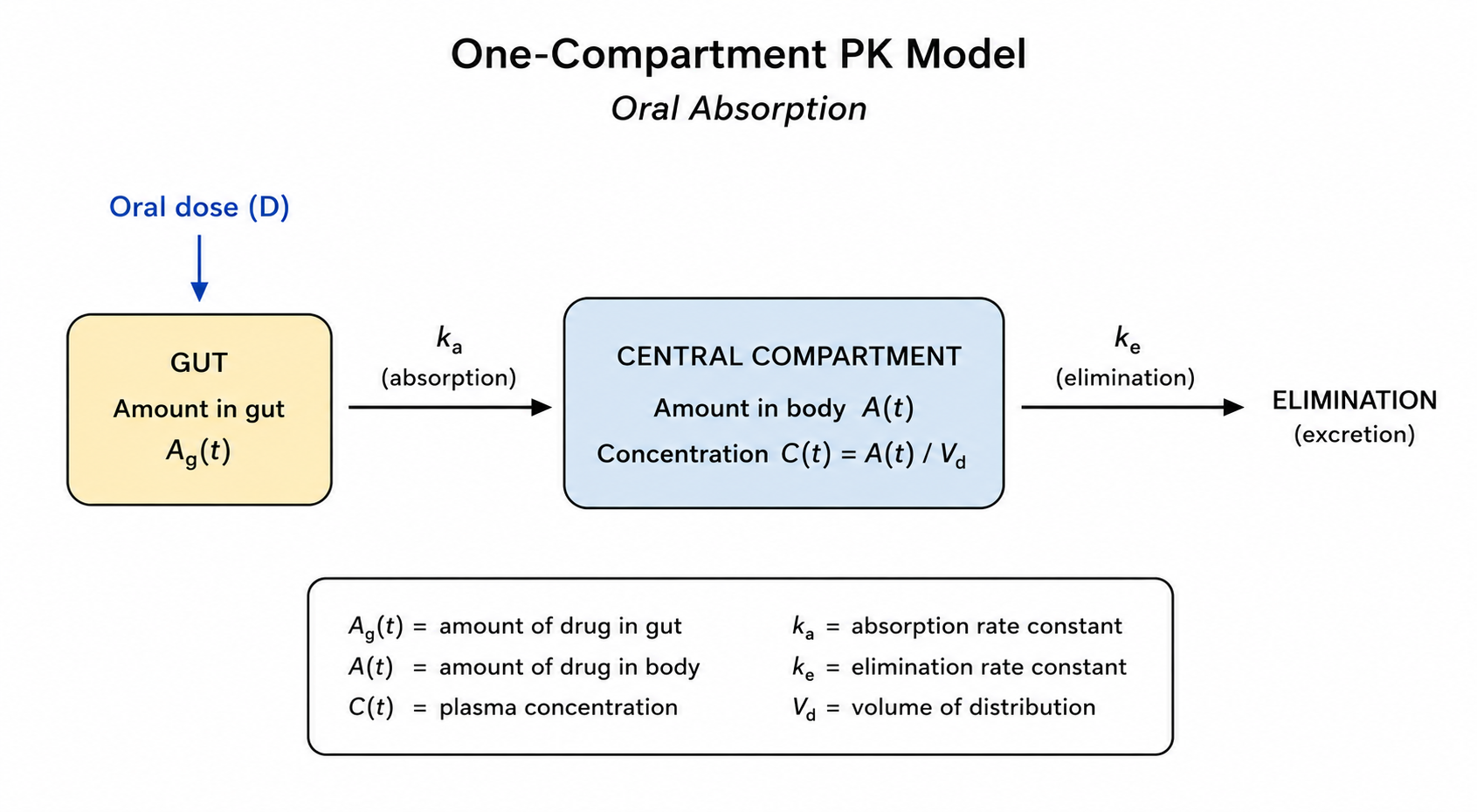
Although the diagram includes a depot/absorption site, the term one-compartment model refers to one systemic disposition compartment: the central compartment.
This model is simple, but it introduces the key modeling logic used throughout population PK.
Worked Example 1: Model Assumptions
A one-compartment oral model usually assumes:
- drug enters through an absorption compartment
- absorption follows first-order kinetics
- the body can be represented by one central compartment
- elimination is linear
- concentration is proportional to the amount in the central compartment
These assumptions are simplifications.
They are useful when they describe the data well enough for the modeling purpose.
Worked Example 2: Concentration-Time Equation
For a single oral dose with first-order absorption and first-order elimination, the concentration-time profile can be written as:
\[ C(t)= \frac{Dose \cdot k_a}{V(k_a-k)} \left( e^{-kt}-e^{-k_a t} \right) \]
where:
\[ k=\frac{CL}{V} \]
Parameter interpretation:
| Parameter | Meaning |
|---|---|
Dose |
administered amount |
ka |
absorption rate constant |
CL |
clearance |
V |
volume of distribution |
k |
elimination rate constant |
This equation predicts the expected concentration at time t.
For simplicity, this equation assumes complete bioavailability. In practice, oral drugs may not reach the systemic circulation completely, which can affect the relationship between dose and concentration.
Note
This equation is an analytic (closed-form) solution for the one-compartment oral PK model under these assumptions.
Because the model has a known mathematical solution, we can compute concentrations directly from the equation.
Later in the course, we will introduce more flexible models that do not have simple closed-form solutions and are instead solved numerically using ordinary differential equations (ODEs), which is one of the strengths of rxode2 and nlmixr2.
Worked Example 3: Simulate One Profile
Define the structural function.
one_comp_oral <- function(time, dose, ka, CL, V) {

  k <- CL / V

  dose * ka / (V * (ka - k)) *
    (exp(-k * time) - exp(-ka * time))
}
Create a time grid and simulate concentrations.
time_grid <- seq(0, 24, length.out = 200)
sim_profile <- tibble(
TIME = time_grid,
CONC = one_comp_oral(
time = time_grid,
dose = 320,
ka = 1,
CL = 3,
V = 30
)
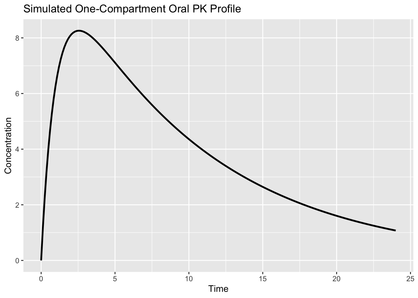
)Plot the simulated profile.
ggplot(sim_profile, aes(TIME, CONC)) +
  geom_line(linewidth = 1) +
  labs(
    title = "Simulated One-Compartment Oral PK Profile",
    x = "Time",
    y = "Concentration"
  )
Worked Example 4: Read the Profile
The profile has three broad regions.
| Region | Interpretation |
|---|---|
| Rising phase | absorption dominates |
| Peak | absorption and elimination are balanced |
| Declining phase | elimination dominates |
This does not mean absorption stops completely after the peak.
It means elimination becomes the dominant visible process.
Worked Example 5: Elimination Rate and Half-Life
The elimination rate constant is:
\[ k=\frac{CL}{V} \]
The half-life is:
\[ t_{1/2}=\frac{\ln(2)}{k} \]
Substituting \(k=CL/V\) gives:
\[ t_{1/2}=\frac{\ln(2)V}{CL} \]
Example calculation:
CL <- 3
V <- 30

k <- CL / V
half_life <- log(2) / k

tibble(
  CL = CL,
  V = V,
  k = k,
  half_life = half_life
)
# A tibble: 1 × 4
CL V k half_life
<dbl> <dbl> <dbl> <dbl>
1 3 30 0.1 6.93Interpretation:
- higher
CLincreaseskand shortens half-life - higher
Vdecreaseskand lengthens half-life
Why This Model Matters
This model is simple enough to understand but powerful enough to introduce core population PK ideas.
Later, we will add:
- random effects
- residual error
- covariates
- estimation with
nlmixr2
For now, the key point is:
The structural equation generates the expected concentration-time profile.
Strategies
- Start with the simplest reasonable model.
- Interpret each parameter biologically.
- Simulate before estimating.
- Use the profile shape to evaluate assumptions.
- Keep structural thinking separate from variability thinking.
Common Mistakes
- Jumping to population estimation too early.
- Ignoring model assumptions.
- Treating the equation as abstract math only.
- Forgetting that oral models require absorption.
- Confusing absorption rate with elimination rate.
Practice Problems
- What does
kacontrol in an oral PK model? - If
CL = 4andV = 40, computek. - If clearance increases while volume stays fixed, what happens to half-life?
- Why does the profile rise before it falls?
- Why is the one-compartment model considered a simplification?
TipStep-by-Step Solutions
Problem 1: What does ka control in an oral PK model?
ka controls the absorption rate from the depot or gut compartment into the central compartment.
A larger ka usually produces faster absorption and an earlier peak concentration.
Problem 2: If CL = 4 and V = 40, compute k.
The elimination rate constant is:
\[ k = \frac{CL}{V} \]
Substitute the values:
\[ k = \frac{4}{40} = 0.1 \]
So the elimination rate constant is 0.1.
Problem 3: If clearance increases while volume stays fixed, what happens to half-life?
Half-life is:
\[ t_{1/2} = \frac{\ln(2)V}{CL} \]
If CL increases and V stays the same, half-life decreases.
The drug is eliminated faster.
Problem 4: Why does the profile rise before it falls?
After oral dosing, drug must first be absorbed into the central compartment.
Early after dosing, absorption can exceed elimination, so concentration rises.
Later, absorption slows and elimination dominates, so concentration falls.
Problem 5: Why is the one-compartment model a simplification?
It represents the body as one kinetically homogeneous disposition compartment.
This is useful, but it ignores more complex behavior such as slow tissue distribution, multiple disposition phases, or nonlinear elimination.
Summary
- The one-compartment oral model is a foundational structural PK model.
ka,CL, andVdetermine profile shape.k = CL / Vconnects clearance and volume to elimination rate.- Half-life depends on both clearance and volume.
- Structural models generate expected concentration-time profiles before variability is added.
TipQuick Tips
kacontrols absorption.CLandVtogether determine elimination rate.- Simulate profiles to understand parameters.
- Structural models come before population variability.