library(tidyverse)
library(nlmixr2)
library(nlmixr2data)

data("theo_sd", package = "nlmixr2data")Interpreting Covariate Effects
Learn how to interpret the size and meaning of covariate effects in population PK models.
Tip
Big picture: Building a covariate model is not enough. We must understand what the estimated effect means biologically.
Learning Objectives
By the end of this lesson, you will be able to:
- interpret covariate effect direction
- interpret covariate effect magnitude
- compare individuals using covariate models
- understand covariate exponents
- distinguish statistical and biological importance
Key Ideas
- sign matters
- magnitude matters
- biology matters
- interpretation matters more than significance
Setup
Why Interpretation Matters
Suppose a model estimates:
\[ TVCL= 3 \left( \frac{WT}{70} \right)^{0.75} \]
Question:
What does 0.75 mean?A parameter estimate becomes useful only after interpretation.
Worked Example 1: Interpret Direction
Suppose:
\[ TVCL= 3 \left( \frac{WT}{70} \right)^{0.75} \]
Interpretation:
- exponent > 0 → clearance increases with weight
- exponent = 0 → no weight effect
- exponent < 0 → clearance decreases with weight
Direction tells us:
Higher Covariate → Higher or Lower ParameterWorked Example 2: Interpret Magnitude
Compare:
\[ TVCL= 3 \left( \frac{WT}{70} \right)^{0.25} \]
vs.
\[ TVCL= 3 \left( \frac{WT}{70} \right)^{1.5} \]
Interpretation:
- \(0.25\) → weaker effect
- \(1.5\) → stronger effect
Larger exponents produce larger parameter changes across the same covariate range.
Worked Example 3: Compare Subjects
Calculate expected clearance for different body weights.
subject_tbl <-
  tibble(
    WT = c(50, 70, 100)
  ) %>%
  mutate(
    TVCL = 3 * (WT / 70)^0.75
  )

subject_tbl
# A tibble: 3 × 2
WT TVCL
<dbl> <dbl>
1 50 2.33
2 70 3
3 100 3.92Visualize the expected differences.
ggplot(subject_tbl, aes(WT, TVCL)) +
  geom_point(size = 3) +
  geom_line() +
  labs(
    title = "Expected Clearance Across Subjects",
    x = "Weight",
    y = "Typical Clearance"
  )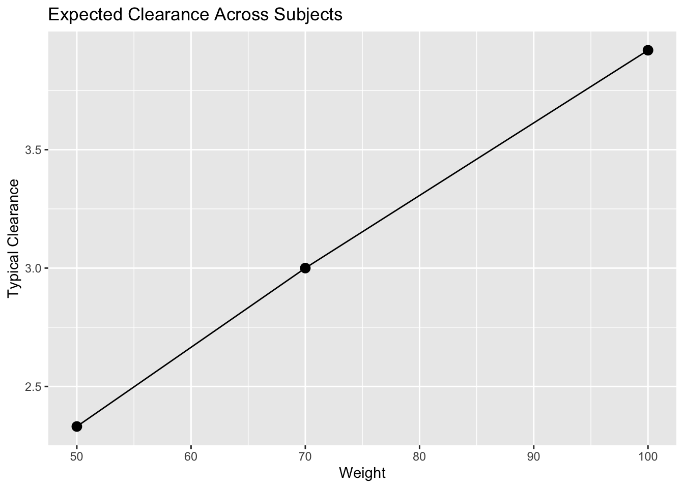
Interpretation:
- all subjects share the same population model
- different weights produce different typical clearance values
- a 100-kg subject is expected to have higher typical clearance than a 50-kg subject
Covariates produce systematic differences between individuals.
Worked Example 4: Continuous vs Categorical Effects
Continuous example:
\[ TVCL= 3 \left( \frac{WT}{70} \right)^{0.75} \]
Interpretation:
Smooth change across weight values.
Categorical example:
\[ TVCL= 3(1+0.2\times SEX) \]
Assume:
- \(SEX=0\) → reference group
- \(SEX=1\) → comparison group
Interpretation:
- \(SEX=0\) → \(TVCL=3\)
- \(SEX=1\) → \(TVCL=3.6\)
The comparison group has 20% higher typical clearance.
Continuous effects change gradually.
Categorical effects change by group.
Worked Example 5: Biological Interpretation
Model:
\[ TVCL= 3 \left( \frac{WT}{70} \right)^{0.75} \]
Question:
Does this make biological sense?Weight often relates to:
- body size
- organ size
- blood flow
- clearance capacity
This helps explain why weight is one of the most common covariates in population PK models.
Interpret parameters mechanistically whenever possible.
Statistical Importance Is Not Enough
Question:
Was an effect detected?Different question:
Is the effect meaningful?Examples:
- statistically significant but clinically trivial
- clinically important but uncertain
- mathematically improved but biologically implausible
Interpretation requires context.
Looking Ahead
We now know how to interpret covariate effects:
Covariate Model → Direction → Magnitude → Biological MeaningNext we connect covariates back to the broader goal of explaining population variability.
Strategies
- compare subjects
- examine effect size
- interpret biologically
- distinguish statistical and clinical meaning
Common Mistakes
- reporting coefficients only
- ignoring units
- ignoring plausibility
- assuming statistical significance means clinical importance
Practice Problems
What does a positive exponent imply?
Compare:
\[ \theta=0.3 \]
vs.
\[ \theta=1.2 \]
- Interpret:
\[ TVCL=3(1+0.2\times SEX) \]
Why are biological explanations important?
Why is statistical significance not enough?
TipStep-by-Step Solutions
Problem 1
A positive exponent means the parameter increases as the covariate increases.
Problem 2
The larger exponent produces a stronger covariate effect across the same covariate range.
Problem 3
The comparison group has 20% higher typical clearance than the reference group.
Problem 4
Biological explanations help determine whether the covariate relationship is plausible and meaningful.
Problem 5
A statistically detected effect may still be too small, uncertain, or implausible to matter clinically.
Summary
- direction tells us whether the parameter increases or decreases
- magnitude tells us how large the effect is
- subject comparisons make covariate effects concrete
- biology matters
- statistical importance is not the same as clinical importance
TipQuick Tips
- Sign matters
- Magnitude matters
- Compare subjects
- Biology matters
- Significance is not enough