library(tidyverse)
library(rxode2)Why Simulate?
Understand why simulation is central to pharmacometric modeling and how it differs from estimation.
Tip
Big picture: Estimation learns from observed data. Simulation uses a model to explore what could happen.
Learning Objectives
By the end of this lesson, you will be able to:
- explain why pharmacometricians simulate
- distinguish estimation from simulation
- describe what-if questions
- understand prediction versus observation
- connect simulation to model-informed decisions
Key Ideas
- estimation uses data to learn model parameters
- simulation uses a model to generate predictions
- simulation explores scenarios
- simulation supports decisions
Setup
This lesson uses a simple simulated PK model.
No estimation is performed.
New Tools Introduced in This Module
This module introduces simulation tools from rxode2.
Think of them as three connected pieces.
| Function | Role |
|---|---|
rxode2() |
defines the model |
et() |
defines events and scenarios |
rxSolve() |
generates simulated outcomes |
Conceptually:
Model

+

Scenario

↓

Simulation
Example:
pk_model <- rxode2(...)

ev <- et(...)

sim <- rxSolve(pk_model, ev)
Interpretation:
rxode2()
↓
Defines system behavior


et()
↓
Defines what happens


rxSolve()
↓
Computes predictions
In later lessons, rxSolve() will also simulate directly from fitted nlmixr2 models.
Estimation versus Simulation
Estimation asks:
Given data, what parameters explain the observations?Simulation asks:
Given a model, what outcomes might occur?Conceptually:
Estimation: Data → Model Parameters

Simulation: Model Parameters → Predicted Outcomes
Both are essential.
They answer different questions.
Why Simulate?
Simulation lets us ask questions that may not be directly answered by the observed data.
Examples:
- What if the dose changes?
- What if dosing happens more often?
- What if patients differ in clearance?
- What response should we expect later?
- What variability should we expect?
Simulation turns a fitted model into a prediction engine.
Worked Example 1: Define a Simple PK Model
Use a one-compartment oral PK model.
pk_model <-
  rxode2({
    ka <- 1
    cl <- 3
    v <- 30

    d/dt(depot) = -ka * depot
    d/dt(center) = ka * depot - cl / v * center

    cp = center / v
  })

pk_model
rxode2 5.1.1 model named rx_f69a20fda9fa08656c71fb657d14e6dd model (✔ ready).
x$state: depot, center
x$params: ka, cl, v
x$lhs: cp
The printed model summarizes the variables and parameters that define the system.
The differential equations describe how drug amount changes in the depot and center compartments over time.
Notice that the output lists:
x$state: depot, center
x$params: ka, cl, v
x$lhs: cpThe states are quantities that change over time according to the differential equations.
The parameters are fixed values used by those equations.
The quantity cp appears under x$lhs because it is a calculated model output:
cp = center / vUnlike depot and center, cp is not a compartment. It is a derived quantity that represents concentration.
Later, when we simulate the model, cp will appear in the simulation output as the predicted concentration.
This model describes:
Dose
↓
Absorption
↓
Central Amount
↓
Concentration
Worked Example 2: Define a Dosing Scenario
Simulation requires a scenario.
Here we simulate a single oral dose.
ev_100 <-
  et(amt = 100, cmt = "depot") %>%
  et(seq(0, 24, by = 0.25)) # add sampling

ev_100
── EventTable with 98 records ──
1 dosing records (see x$get.dosing(); add with add.dosing or et)
97 observation times (see x$get.sampling(); add with add.sampling or et)
── First part of x: ──
# A tibble: 98 × 4
time cmt amt evid
<dbl> <chr> <dbl> <evid>
1 0 depot 100 1:Dose (Add)
2 0 <NA> NA 0:Observation
3 0.25 <NA> NA 0:Observation
4 0.5 <NA> NA 0:Observation
5 0.75 <NA> NA 0:Observation
6 1 <NA> NA 0:Observation
7 1.25 <NA> NA 0:Observation
8 1.5 <NA> NA 0:Observation
9 1.75 <NA> NA 0:Observation
10 2 <NA> NA 0:Observation
# ℹ 88 more rowsThe printed event table summarizes the simulation scenario.
Notice that it contains:
- one dosing record
- multiple observation times
The dosing record specifies what happens to the virtual subject:
100 mg dose into the depot compartment at time 0The observation records specify when model predictions should be returned.
In this example, predictions are requested every 0.25 hours from 0 to 24 hours.
Because cp was defined as a model output, concentration predictions for cp will be returned at each observation time.
Interpretation:
100 mg dose → predict concentration over 24 hoursThe event table defines what happens to the virtual subject and when model predictions are requested.
Worked Example 3: Simulate Concentration
Run the simulation.
sim_100 <-
  rxSolve(pk_model, ev_100) %>%
  as_tibble()
Inspect the output.
sim_100 %>% head()# A tibble: 6 × 4
time cp depot center
<dbl> <dbl> <dbl> <dbl>
1 0 0 100 0
2 0.25 0.728 77.9 21.8
3 0.5 1.28 60.7 38.3
4 0.75 1.69 47.2 50.6
5 1 1.99 36.8 59.7
6 1.25 2.21 28.7 66.2The simulation output is a dataset.
Each row corresponds to a time point from the event table.
The column cp appears because we defined it in the model as:
cp = center / vSo cp is the predicted concentration returned by the simulation.
Plot the concentration profile.
ggplot(sim_100, aes(time, cp)) +
    geom_line() +
    labs(
        title = "Simulated Concentration After 100 mg",
        x = "Time",
        y = "Concentration"
    )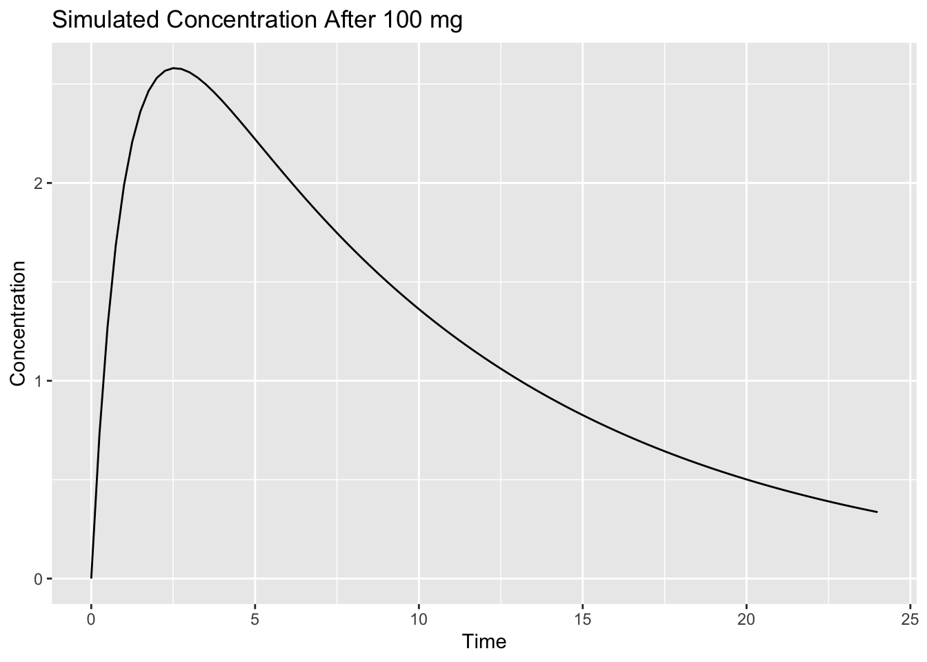
Interpretation:
The model generates concentration values over time.
These are predictions, not observations.
Worked Example 4: Ask a What-If Question
Now ask:
What if the dose were higher?
Simulate 200 mg.
ev_200 <-
  et(amt = 200, cmt = "depot") %>%
  et(seq(0, 24, by = 0.25))

sim_200 <-
  rxSolve(pk_model, ev_200) %>%
  as_tibble()
This uses the same model and the same sampling schedule.
Only the dose amount has changed.
This is what makes the example a clean what-if comparison.
Combine scenarios.
sim_compare <-
  bind_rows(
    sim_100 %>% mutate(DOSE = "100 mg"),
    sim_200 %>% mutate(DOSE = "200 mg")
  )
The DOSE column labels each simulated scenario so they can be compared in one plot.
Plot.
ggplot(sim_compare, aes(time, cp, linetype = DOSE)) +
    geom_line() +
    labs(
        title = "Dose Scenario Comparison",
        x = "Time",
        y = "Concentration"
    )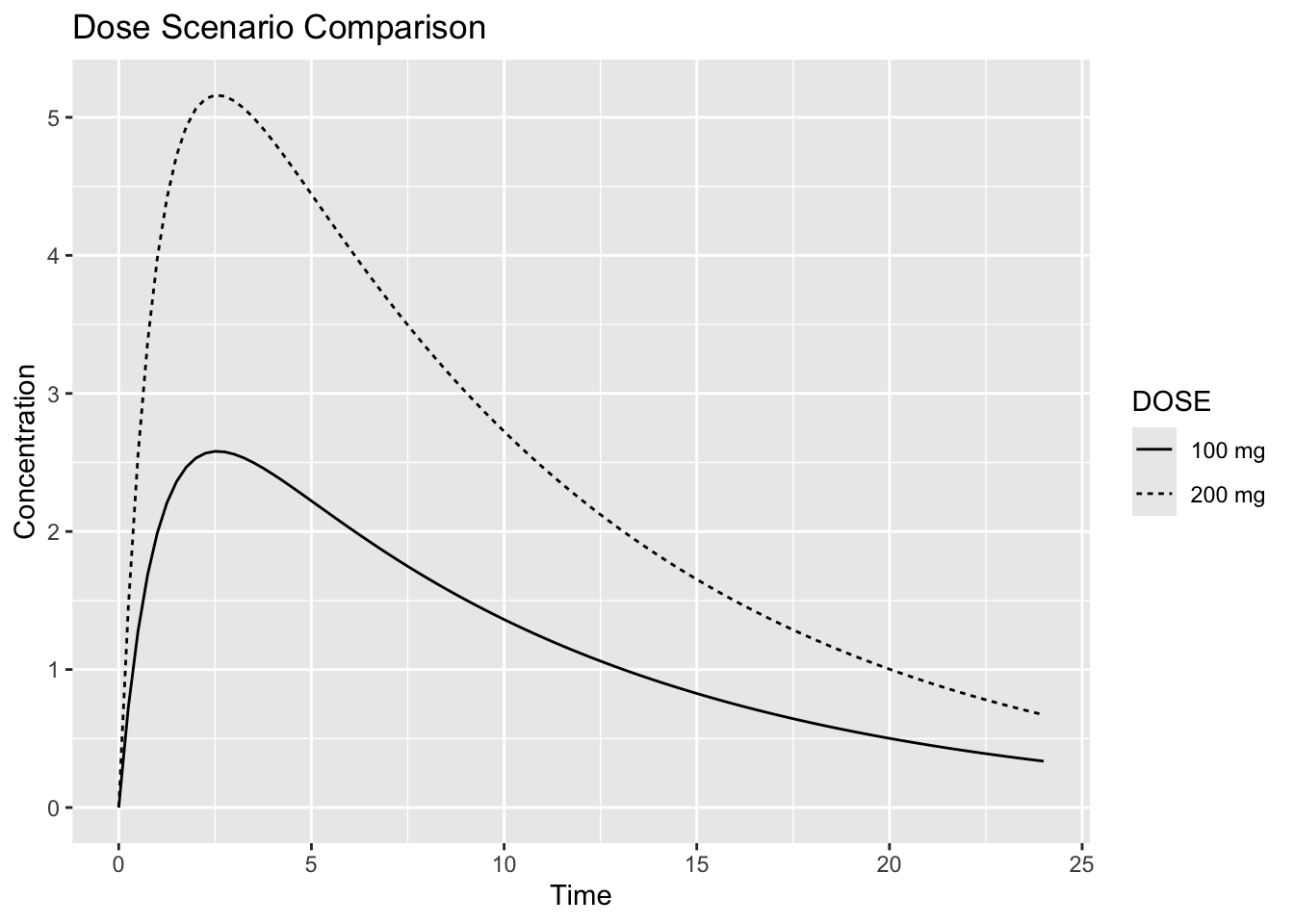
Interpretation:
Simulation lets us compare scenarios before observing them directly.
In this simple linear PK model, increasing the dose increases predicted concentration while keeping the overall profile shape similar.
Worked Example 5: Simulation Supports Decisions
Simulation does not make decisions automatically.
It provides evidence.
Conceptually:
Model

↓

Scenario

↓

Simulation

↓

Interpretation

↓

Decision
Examples:
| Question | Simulation Output |
|---|---|
| Does exposure increase? | concentration-time profiles |
| Is accumulation expected? | repeated-dose profiles |
| Do patients differ? | population simulations |
| Which strategy looks better? | scenario comparison |
A simulation is only as useful as the model and assumptions behind it.
What Simulation Does Not Prove
Simulation does not prove the future.
It depends on:
- model structure
- parameter estimates
- assumptions
- variability
- scenario definition
Simulation is best interpreted as:
Model-based expectationnot guaranteed truth.
Looking Ahead
This lesson used a simple typical-subject simulation.
Next, we add variability.
We will compare:
Typical Individual
↓
Population of Individuals
Strategies
- define the question first
- simulate simple scenarios before complex ones
- interpret outputs in context
Common Mistakes
- treating simulation as proof
- forgetting variability
- changing too many assumptions at once
Practice Problems
What question does estimation answer?
What question does simulation answer?
Why do simulations need a scenario?
What is the difference between prediction and observation?
Why should simulation results be interpreted cautiously?
TipStep-by-Step Solutions
Problem 1
Estimation asks:
Given data, what parameters explain the observations?Problem 2
Simulation asks:
Given a model, what outcomes might occur?Problem 3
A scenario defines what is being simulated.
Examples include dose, timing, patient characteristics, and sampling times.
Problem 4
A prediction is generated by a model.
An observation is measured from real data.
Problem 5
Simulation depends on assumptions.
If the model or scenario is unrealistic, the simulation may be misleading.
Summary
- estimation learns from data
- simulation explores scenarios
- simulation generates model-based predictions
- interpretation depends on assumptions
TipQuick Tips
- Estimate first
- Simulate scenarios
- Interpret cautiously
- Models support decisions