library(tidyverse)
library(nlmixr2data)

data("theo_sd", package = "nlmixr2data")

theo <- theo_sd

obs <- theo %>%
  filter(EVID == 0)

dose <- theo %>%
filter(EVID != 0)From Data to Modeling Dataset
Consolidate exploratory analysis and prepare a reviewed dataset for structural PK modeling.
Tip
Big picture: Before building equations, we should pause and confirm that the dataset has been reviewed and that the next step is truly modeling—not more cleaning.
Learning Objectives
By the end of this lesson, you will be able to:
- Consolidate dataset understanding.
- Review event records and observations.
- Summarize exploratory findings.
- Create a reusable modeling object.
- Identify readiness for structural modeling.
Key Ideas
- EDA should lead to decisions.
- Modeling datasets should be reviewed before estimation.
- Visualization generates hypotheses.
- Modeling starts after understanding the data.
Setup
What We Learned from the Dataset
At this point, we already know:
- the dataset uses event records
- observations and doses coexist
- concentrations follow expected PK behavior
- subjects show variability
- weight varies across subjects
- event ordering appears reasonable
The goal now is to consolidate—not rediscover.
Worked Example 1: Build a Modeling Summary
Create a compact dataset summary.
dataset_summary <-
tibble(
  n_subjects =
    n_distinct(theo$ID),

  n_rows =
    nrow(theo),

  n_observations =
    nrow(obs),

  n_dose_rows =
    nrow(dose),

  min_time =
    min(obs$TIME),

  max_time =
    max(obs$TIME)
)

dataset_summary
# A tibble: 1 × 6
n_subjects n_rows n_observations n_dose_rows min_time max_time
<int> <int> <int> <int> <dbl> <dbl>
1 12 144 132 12 0 24.6Worked Example 2: Build a Modeling Object
Create a reviewed modeling object.
theo_model <-
theo %>%
  arrange(ID, TIME)

head(theo_model)
ID TIME DV AMT EVID CMT WT
1 1 0.00 0.00 319.992 101 1 79.6
2 1 0.00 0.74 0.000 0 2 79.6
3 1 0.25 2.84 0.000 0 2 79.6
4 1 0.57 6.57 0.000 0 2 79.6
5 1 1.12 10.50 0.000 0 2 79.6
6 1 2.02 9.66 0.000 0 2 79.6Confirm dimensions.
dim(theo_model)[1] 144 7This object will serve as the working dataset in later modules.
No rows were removed.
No transformations were applied.
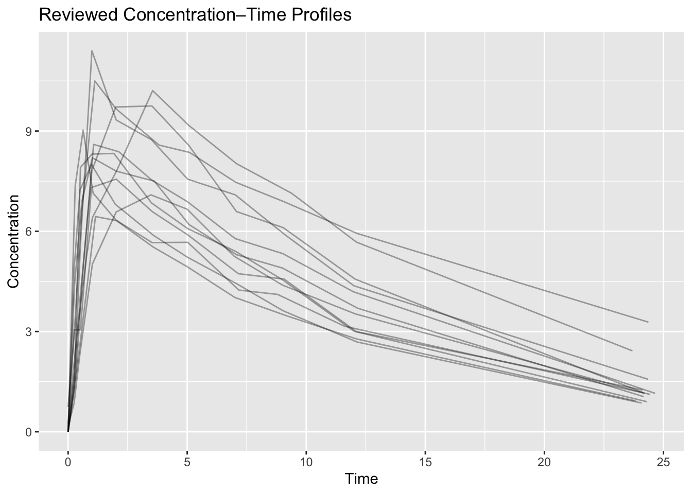
Worked Example 3: Final Concentration Profile
Generate one final subject-level plot.
ggplot(
  obs, aes(TIME, DV, group = ID)) +
    geom_line(alpha = 0.35) +
    labs(
        title = "Reviewed Concentration–Time Profiles",
        x = "Time",
        y = "Concentration"
    )
Ask:
- Does concentration behave reasonably?
- Is variability visible?
- Are observations plausible?
If yes, proceed.
Worked Example 4: Readiness Checklist
Create a simple readiness table.
readiness <-
tibble(
  check = c(
    "Events reviewed",
    "Observations inspected",
    "Profiles visualized",
    "Dose records reviewed",
    "Working dataset created"
  ),
  status = "Complete"
)

readiness
# A tibble: 5 × 2
check status
<chr> <chr>
1 Events reviewed Complete
2 Observations inspected Complete
3 Profiles visualized Complete
4 Dose records reviewed Complete
5 Working dataset created CompleteTransition to Structural Modeling
Until now we have focused on:
Data
↓
QC
↓
Visualization
The next module introduces:
Data
↓
Structural PK Model
↓
Parameters
↓
Predictions
This is where equations begin.
Strategies
- Review findings.
- Freeze assumptions.
- Move forward intentionally.
Common Mistakes
- Repeating QC endlessly.
- Changing datasets during estimation.
- Losing reproducibility.
Practice Problems
- Recreate the summary table.
- Create a reviewed modeling object.
- Write three observations about the concentration profiles.
- Explain why modeling has not started yet.
TipStep-by-Step Solutions
Reuse the code blocks above.
Focus on interpretation and readiness—not additional cleaning.
Summary
- You reviewed
theo_sd. - You explored event records.
- You visualized concentration profiles.
- You created a modeling object.
- You are ready for structural PK modeling.
TipQuick Tips
- Understand first.
- Model second.
- Keep datasets stable.
- Use plots to ask questions.