library(tidyverse)
library(nlmixr2)
library(nlmixr2data)

data("theo_sd", package = "nlmixr2data")Why Model Diagnostics Matter
Understand why estimation alone is not enough and learn the role of diagnostics in population PK modeling.
Tip
Big picture: Diagnostics do not build models. Diagnostics evaluate whether the assumptions used to build the model remain reasonable after fitting.
Learning Objectives
By the end of this lesson, you will be able to:
- explain why diagnostics are needed after estimation
- distinguish convergence from model adequacy
- connect diagnostics to model assumptions
- describe the role of predictions and residuals
- prepare for formal diagnostic plots
Key Ideas
- estimation and diagnostics answer different questions
- diagnostics evaluate assumptions
- convergence does not guarantee adequacy
- diagnostics support decision making
Setup
Fit the model.
one_comp_model <- function(){

    ini({

        tka <- log(1)
        tcl <- log(3)
        tv <- log(30)

        eta.ka ~ 0.1
        eta.cl ~ 0.1
        eta.v ~ 0.1

        add.err <- 0.1

    })

    model({

        ka <- exp(tka + eta.ka)

        cl <- exp(tcl + eta.cl)

        v <- exp(tv + eta.v)

        linCmt() ~ add(add.err)

    })

}

fit <-
  nlmixr2(
    one_comp_model,
    theo_sd,
    est = "focei",
    control = list(print = 0)
  )

fit_tbl <-
  fit %>%
  as_tibble()
Diagnostics in the Population Modeling Workflow
Diagnostics are used throughout population model development.
After fitting a model, we evaluate whether the model assumptions and predictions appear reasonable before deciding whether additional model refinement is needed.
For example, diagnostics may be reviewed after:
Structural Model

↓

Variability Model

↓

Covariate Model

↓

Final Model
and after any major model modification.
Their purpose is evaluation.
Diagnostics ask:
Did our assumptions behave reasonably?
Throughout this module, we will learn how diagnostic tools help identify model strengths, reveal potential problems, and guide model improvement.
Why Diagnostics Matter
Model fitting answers:
What parameter values best explain the data?
Diagnostics answer:
Did the model explain the data reasonably while preserving reasonable assumptions?
Diagnostics evaluate:
- structural assumptions
- variability assumptions
- covariate assumptions
- residual assumptions
A model may:
- converge
- estimate parameters
- produce predictions
and still be inadequate.
Worked Example 1: Convergence Is Not Enough
Suppose two models both converge.
Model A:
- unbiased predictions
- stable residuals
Model B:
- systematic underprediction
- structured residual patterns
Only diagnostics reveal the difference.
Question:
Did the issue originate from:
- structure?
- variability?
- covariates?
- residual error?
Diagnostics help narrow the answer.
Worked Example 2: Inspect Predictions
Inspect prediction quantities.
fit_tbl %>%
  select(
    DV,
    PRED,
    IPRED
  ) %>%
  head()
# A tibble: 6 × 3
DV PRED IPRED
<dbl> <dbl> <dbl>
1 0.74 0 0
2 2.84 3.26 3.85
3 6.57 5.83 6.78
4 10.5 7.87 9.04
5 9.66 8.51 9.79
6 8.58 7.62 9.09Interpretation:
| Variable | Meaning |
|---|---|
| DV | observed concentration |
| PRED | population prediction |
| IPRED | individual prediction |
These quantities become the foundation of diagnostics.
Worked Example 3: Preview Model Agreement
ggplot(
  fit_tbl,
  aes(PRED, DV)
) +
geom_point(alpha = 0.35) +
geom_abline(
  slope = 1,
  intercept = 0,
  linetype = 2
) +
labs(
  title = "Observed vs Population Prediction",
  x = "PRED",
  y = "DV"
)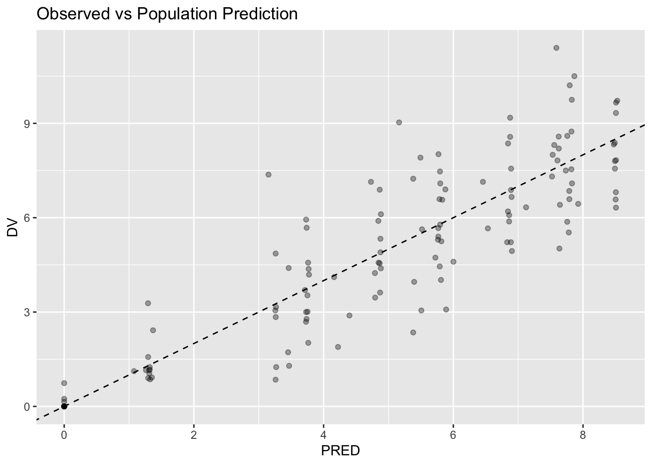
Interpretation:
- points closer to the line suggest stronger agreement
- scatter is expected
- diagnostics evaluate patterns, not perfection
Agreement alone is not enough.
Patterns may indicate:
- missing structure
- incorrect variability
- missing covariates
Worked Example 4: Inspect Residuals
fit_tbl %>%
  select(
    DV,
    PRED,
    RES
  ) %>%
  head()
# A tibble: 6 × 3
DV PRED RES
<dbl> <dbl> <dbl>
1 0.74 0 0.74
2 2.84 3.26 -0.422
3 6.57 5.83 0.740
4 10.5 7.87 2.63
5 9.66 8.51 1.15
6 8.58 7.62 0.955Residual:
\[ Residual= Observed- Predicted \]
Visualize residual behavior.
ggplot(
  fit_tbl,
  aes(PRED, RES)
) +
geom_point(alpha = 0.35) +
geom_hline(
  yintercept = 0,
  linetype = 2
) +
labs(
  title = "Residuals vs Population Prediction",
  x = "PRED",
  y = "RES"
)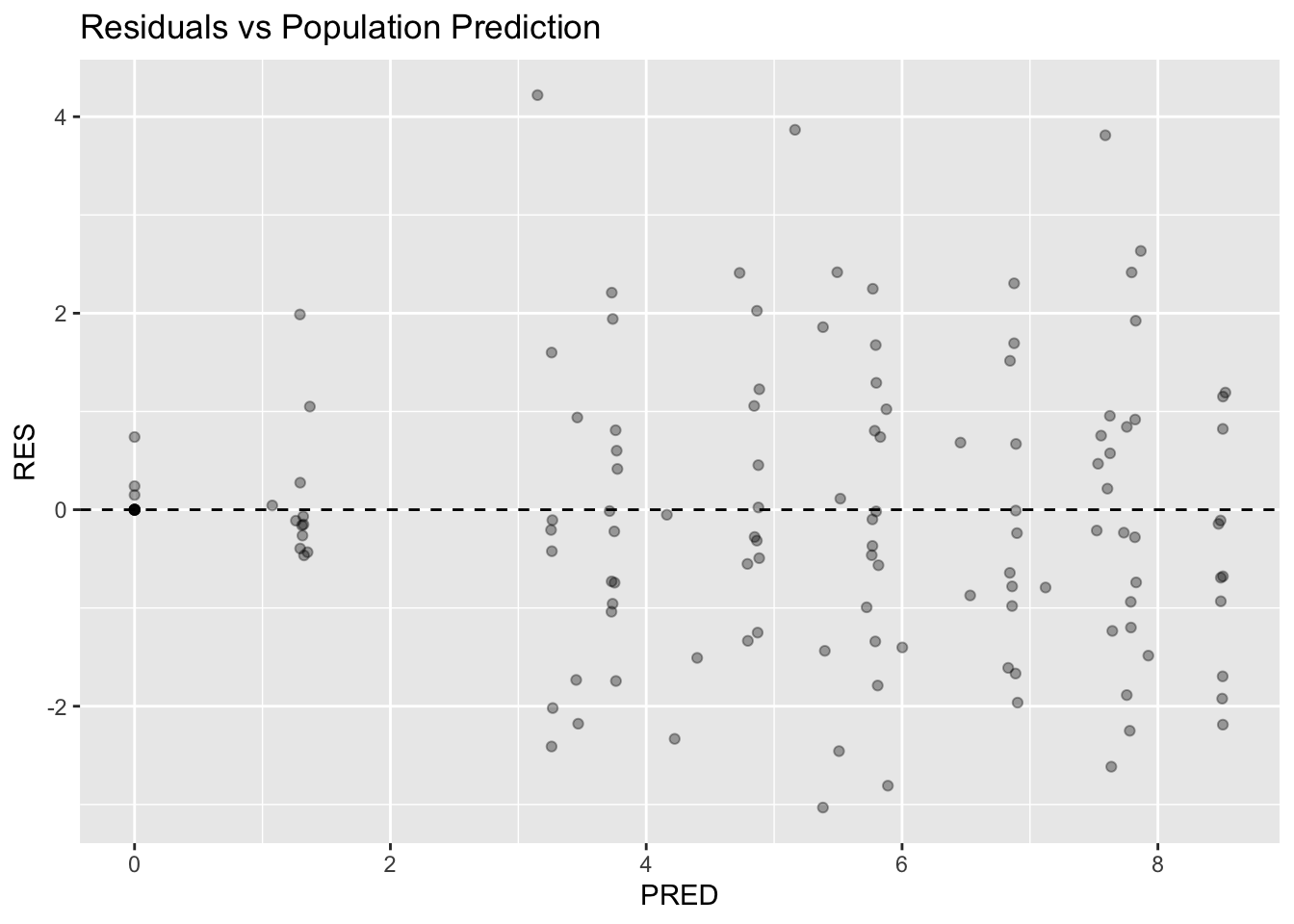
Interpretation:
- residuals should be roughly centered
- systematic trends suggest problems
Residual behavior reflects:
Prediction Quality + Residual AssumptionsRecall that we previously introduced:
- additive residual variability
- proportional residual variability
- combined residual variability
Diagnostics help evaluate whether those assumptions appear reasonable.
Formal residual diagnostics come later.
Worked Example 5: Diagnostic Workflow
Structural Model

↓

Population Model

↓

Variability

↓

Covariates

↓

Predictions

↓

Residuals

↓

Diagnostics

↓

Decision
Diagnostics do not create models.
Diagnostics evaluate models.
Note
In this lesson, we created simple plots directly from model output to understand diagnostic concepts.
Starting in the next lesson, we will begin using ggPMX, which provides standardized pharmacometric diagnostics.
What Diagnostics Cannot Tell Us
Diagnostics do not prove:
- biological truth
- causality
- clinical utility
Diagnostics support judgment.
They do not replace judgment.
Strategies
- inspect before concluding
- compare observations and predictions
- study patterns
Common Mistakes
- treating estimation as validation
- overinterpreting one plot
- ignoring systematic trends
Practice Problems
Why are diagnostics needed?
Why does convergence not guarantee adequacy?
Interpret one residual.
Create DV vs PRED and describe agreement.
Name one thing diagnostics evaluate.
TipStep-by-Step Solutions
Problem 1
Diagnostics evaluate whether assumptions remain reasonable.
Problem 2
Convergence means optimization finished.
It does not guarantee:
- realistic predictions
- realistic variability
- absence of bias
Problem 3
Positive residual:
Observed > PredictedNegative residual:
Observed < PredictedProblem 4
Ask:
- Is agreement reasonable?
- Is there structure?
Problem 5
Diagnostics evaluate:
Structure

↓

Variability

↓

Residuals

↓

Adequacy
Summary
- estimation and diagnostics answer different questions
- diagnostics evaluate assumptions
- predictions and residuals support evaluation
- diagnostics support decisions
TipQuick Tips
- Convergence ≠ adequacy
- Evaluate assumptions
- Residuals matter
- Patterns matter