library(tidyverse)
library(nlmixr2)
library(nlmixr2data)
library(ggPMX)

data("theo_sd", package = "nlmixr2data")Residual Diagnostics
Use residual diagnostics to identify bias, trends, and model inadequacy using ggPMX and nlmixr2.
Tip
Big picture: Residual diagnostics evaluate whether the residual assumptions introduced earlier remain reasonable after fitting.
Learning Objectives
By the end of this lesson, you will be able to:
- Distinguish common residual quantities.
- Interpret residual diagnostic plots.
- Generate residual diagnostics using
ggPMX. - Recognize signs of bias.
- Explain why residuals are central to model evaluation.
Key Ideas
- Residuals measure disagreement.
- Random residuals are preferred.
- Patterns often suggest model issues.
- Diagnostics focus on trends rather than isolated observations.
Setup
Fit the model.
one_comp_model <- function(){

    ini({

        tka <- log(1)
        tcl <- log(3)
        tv <- log(30)

        eta.ka ~ 0.1
        eta.cl ~ 0.1
        eta.v ~ 0.1

        add.err <- 0.1

    })

    model({

        ka <- exp(tka + eta.ka)
        cl <- exp(tcl + eta.cl)
        v <- exp(tv + eta.v)

        linCmt() ~ add(add.err)

    })

}

fit <-
nlmixr2(
  one_comp_model,
  theo_sd,
  est = "focei",
  control = list(
    print = 0
  )
)

fit_tbl <-
fit %>%
as_tibble()

ctr <- pmx_nlmixr(fit)
Why Residual Diagnostics Matter
Residual diagnostics evaluate:
Observed

↓

Prediction

↓

Residual

↓

Residual Assumptions
Residuals should ideally behave randomly.
Residual diagnostics evaluate whether assumptions about residual variability remain reasonable.
Earlier we introduced:
- additive residual variability
- proportional residual variability
- combined residual variability
Residual diagnostics help evaluate those assumptions.
Patterns may suggest:
- structural problems
- incorrect residual assumptions
- unexplained variability
- time-dependent bias
Worked Example 1: Inspect Residual Variables
Inspect residual quantities stored in the fit.
fit_tbl %>%
  select(
    DV,
    PRED,
    RES,
    WRES,
    IRES,
    IWRES,
    CWRES
  ) %>%
  head()
# A tibble: 6 × 7
DV PRED RES WRES IRES IWRES CWRES
<dbl> <dbl> <dbl> <dbl> <dbl> <dbl> <dbl>
1 0.74 0 0.74 1.07 0.74 1.07 1.07
2 2.84 3.26 -0.422 -0.225 -1.01 -1.45 -0.177
3 6.57 5.83 0.740 0.297 -0.215 -0.310 0.287
4 10.5 7.87 2.63 1.23 1.46 2.10 1.17
5 9.66 8.51 1.15 0.826 -0.125 -0.180 0.760
6 8.58 7.62 0.955 0.805 -0.514 -0.741 0.723Interpretation:
| Variable | Meaning |
|---|---|
| RES | observed − population prediction |
| WRES | weighted residual |
| IRES | observed − individual prediction |
| IWRES | individual weighted residual |
| CWRES | conditional weighted residual |
We will focus primarily on CWRES.
Residual Types in Population Modeling
Residual quantities differ in how disagreement is scaled.
Simple residual:
\[ RES = DV - PRED \]
Interpretation:
Observed − Population PredictionWeighted residual:
\[ WRES = \frac{DV - PRED}{\text{Estimated Residual Variability}} \]
Interpretation:
Disagreement
adjusted for expected noise
Large positive values:
Observed much higher than expectedLarge negative values:
Observed much lower than expectedIndividual weighted residual:
\[ IWRES = \frac{DV - IPRED}{\text{Estimated Residual Variability}} \]
Interpretation:
Disagreement relative to the individual predictionConditional weighted residual:
\[ CWRES \approx \frac{DV - E(DV)}{SD(DV)} \]
Interpretation:
Observed disagreement
adjusted using the fitted population model
CWRES accounts for:
- fixed effects
- variability
- residual error
Because of this, CWRES is commonly preferred for diagnostics.
Question:
Why not use simple residuals?
Because residual magnitude often changes with:
- concentration
- variability
- uncertainty
CWRES standardizes disagreement and allows more meaningful comparison across observations.
Worked Example 2: CWRES vs Population Prediction
pmx_plot_cwres_pred(ctr)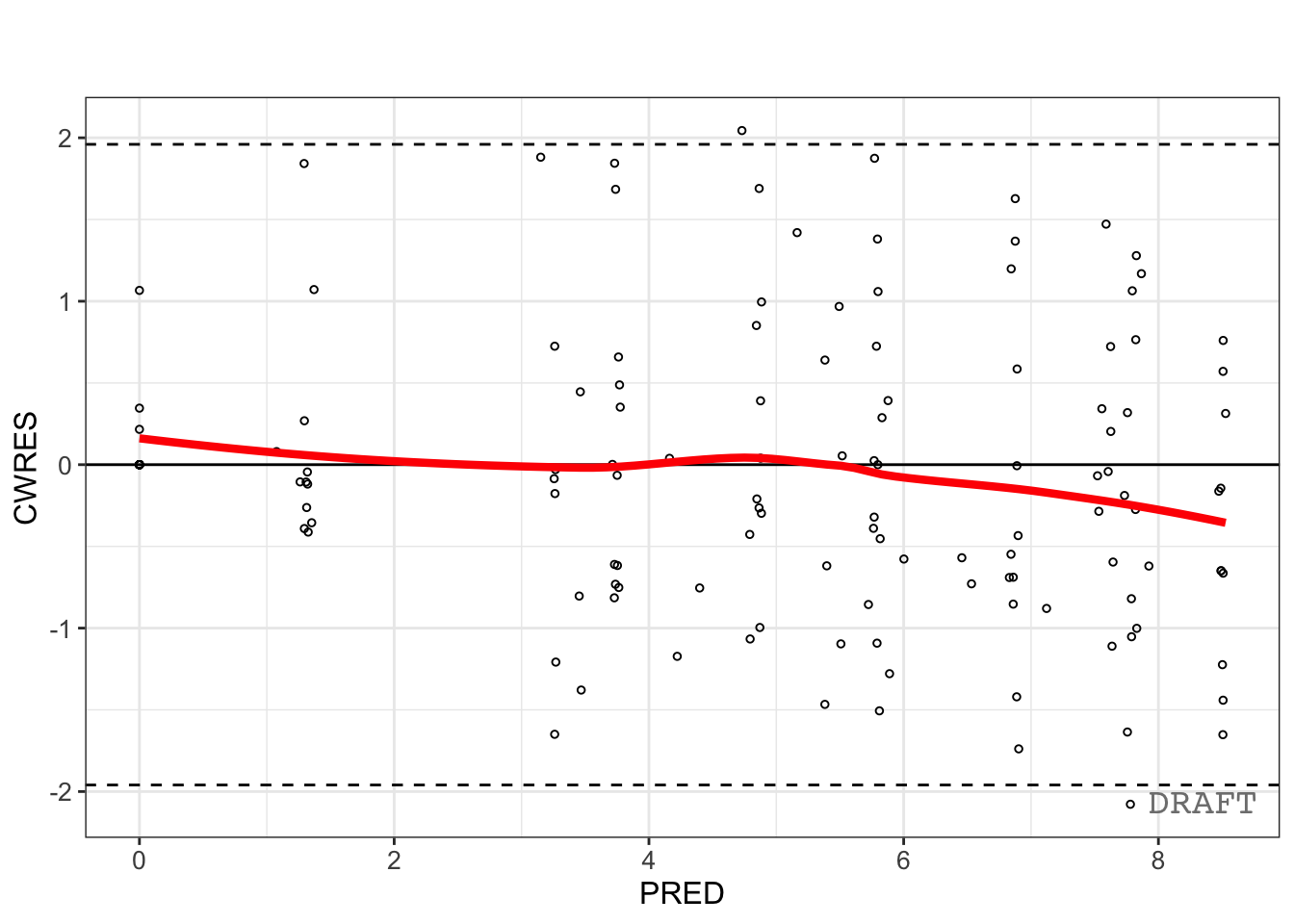
Interpretation:
Look for:
- residuals centered around zero
- absence of obvious trends
- relatively stable spread
Possible concerns:
- curvature
- increasing spread
- clusters
Worked Example 3: CWRES vs Time
pmx_plot_cwres_time(ctr)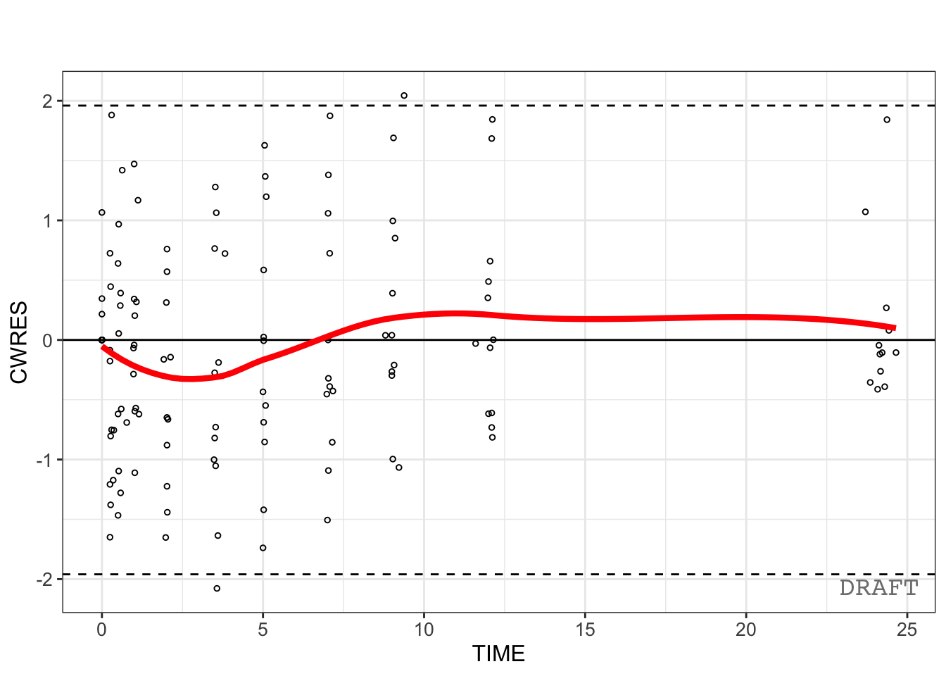
Interpretation:
Look for:
- drift over time
- changing variability
- delayed bias
Residual patterns over time may indicate model misspecification.
Worked Example 4: Inspect the Residual Distribution
Residuals should not only appear random across prediction and time.
Their distribution also matters.
Build a residual histogram manually.
ggplot(
  fit_tbl,
  aes(CWRES)
) +
geom_histogram(
  bins = 20
) +
labs(
  title = "CWRES Distribution",
  x = "CWRES",
  y = "Count"
)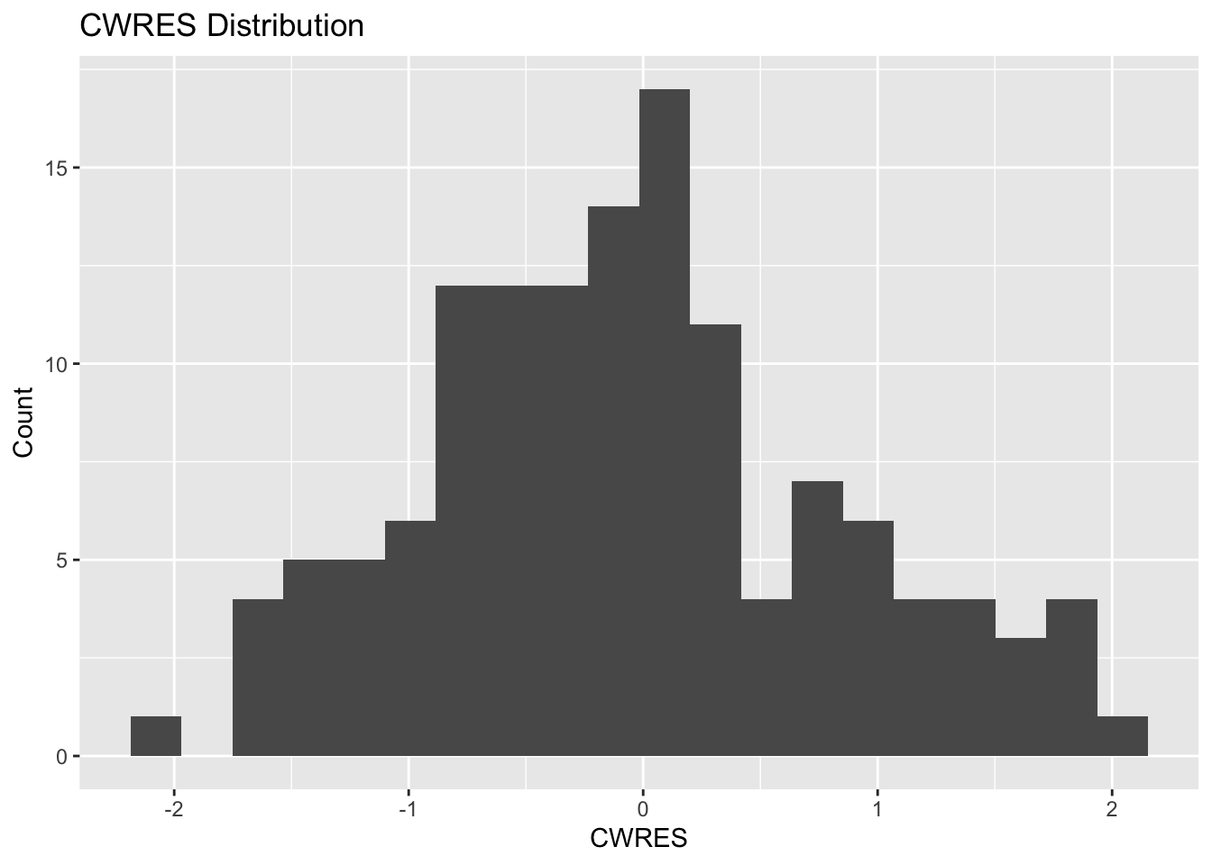
Interpretation:
Look for:
- approximate centering near zero
- reasonable symmetry
- absence of extreme tails
Question:
Do residuals behave approximately as expected?Residual distributions support residual assumptions.
Worked Example 5: Build One Residual Plot Manually
Although ggPMX provides standardized diagnostics, understanding the underlying variables helps interpretation.
ggplot(
  fit_tbl,
  aes(PRED, CWRES)
) +
geom_point(
  alpha = 0.35
) +
geom_hline(
  yintercept = 0,
  linetype = 2
) +
labs(
  title = "CWRES vs Population Prediction",
  x = "PRED",
  y = "CWRES"
)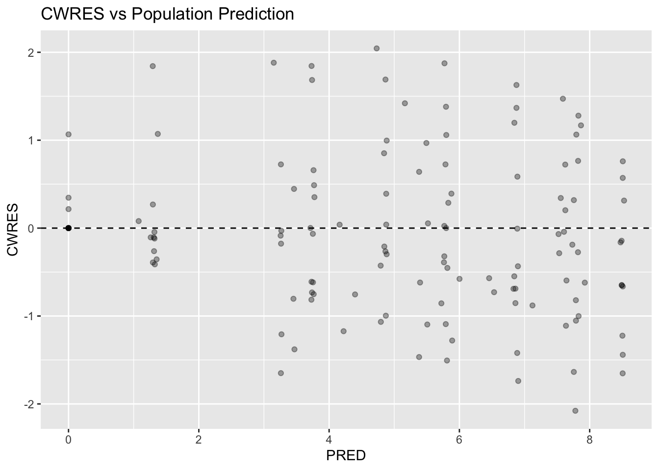
Manual plots and standardized plots should tell a consistent story.
Worked Example 6: Residual Interpretation Framework
Review residual diagnostics in order:
Centering

↓

Trend

↓

Spread

↓

Distribution

↓

Outliers

↓

Model Issue?
Ask:
- residual assumption problem?
- structural problem?
- missing covariates?
- unexplained variability?
Avoid conclusions from isolated points.
Strategies
- inspect multiple diagnostics
- compare residual definitions
- focus on overall behavior
Common Mistakes
- expecting residuals to equal zero
- diagnosing from one point
- confusing variability with bias
Practice Problems
What does CWRES represent?
Why are residual plots centered around zero?
Generate:
pmx_plot_cwres_pred(
  ctr
)
Describe one observation.
- Generate:
pmx_plot_cwres_hist(ctr)Describe:
- centering
- spread
- symmetry
- Why are residual diagnostics useful after GOF plots?
TipStep-by-Step Solutions
Problem 1
CWRES is:
Observed − Expected
scaled by model uncertainty
It standardizes disagreement.
Problem 2
Residual plots are centered around zero because:
Positive Errors

↓

Negative Errors
should balance.
Problem 3
Generate:
pmx_plot_cwres_pred(ctr)
Inspect:
- centering
- spread
- trends
Ask:
Random
or
Structured?
Problem 4
Generate:
pmx_plot_cwres_time(
  ctr
)
Inspect:
- drift
- changing variability
- delayed bias
Problem 5
Multiple diagnostics are needed because:
GOF

↓

Residuals

↓

VPC
each evaluates different model behavior.
Summary
- residual diagnostics evaluate disagreement
- residual diagnostics evaluate residual assumptions
- CWRES is commonly preferred
- trends matter more than isolated observations
- diagnostics should be interpreted collectively
TipQuick Tips
- Centered is better
- Patterns > points
- Inspect more than one diagnostic