library(tidyverse)
library(nlmixr2)
library(nlmixr2data)
library(nlmixr2plot)

data("theo_sd", package = "nlmixr2data")Visual Predictive Checks
Use simulation-based diagnostics to evaluate whether the model reproduces observed variability.
Tip
Big picture: Good predictions are not enough.
A model should reproduce:
- central tendency
- variability
- covariate behavior
- residual behavior.
Learning Objectives
By the end of this lesson, you will be able to:
- Explain the purpose of a Visual Predictive Check (VPC).
- Distinguish predictions from simulations.
- Generate a VPC using
nlmixr2simulation diagnostics. - Interpret simulated intervals relative to observations.
- Recognize common VPC warning signs.
Key Ideas
- VPCs are simulation-based diagnostics.
- Diagnostics evaluate both central tendency and variability.
- Observations are compared against simulated prediction intervals.
- Agreement is evaluated visually.
Setup
Fit the model.
one_comp_model <- function(){

  ini({

    tka <- log(1)
    tcl <- log(3)
    tv <- log(30)

    eta.ka ~ 0.1
    eta.cl ~ 0.1
    eta.v ~ 0.1

    add.err <- 0.1

  })

  model({

    ka <- exp(tka + eta.ka)

    cl <- exp(tcl + eta.cl)

    v <- exp(tv + eta.v)

    linCmt() ~ add(add.err)

  })

}

fit <-
  nlmixr2(
    one_comp_model,
    theo_sd,
    est = "focei",
    control = list(
      print = 0
    )
  )
This fitted model will now be used to generate simulated studies for VPC evaluation.
Why Visual Predictive Checks Matter
Earlier diagnostics asked:
GOF → Do predictions agree?

Residual Diagnostics → Do residual assumptions behave reasonably?
Visual Predictive Checks (VPCs) add another question:
Can the model reproduce observed variability?
Unlike earlier diagnostics, VPCs evaluate simulated studies rather than a single set of predictions.
Conceptually:
Observed Data
→ Simulate New Studies
→ Generate Prediction Intervals
→ Compare Observed vs Simulated
→ Model Evaluation
This changes the focus.
GOF → Observed vs Prediction

Residual Diagnostics → Observed vs Prediction Error

VPC → Observed vs Simulated Data
This makes VPC a broader diagnostic.
VPC evaluates the combined result of:
- structural assumptions
- variability assumptions
- covariate assumptions
- residual assumptions
Question:
If the fitted model were true,
would data like ours commonly occur?
This is why VPC appears later in the workflow.
Structure
→ Variability
→ Covariates
→ GOF
→ Residuals
→ VPC
→ Qualification
VPC evaluates the entire model rather than a single component.
Worked Example 1: Generate a Visual Predictive Check
Generate a Visual Predictive Check (VPC).
Unlike previous diagnostics, a VPC does not compare observations directly to a single prediction.
Instead, it repeatedly simulates new datasets from the fitted model and asks:
If this model were true, would data like ours commonly occur?
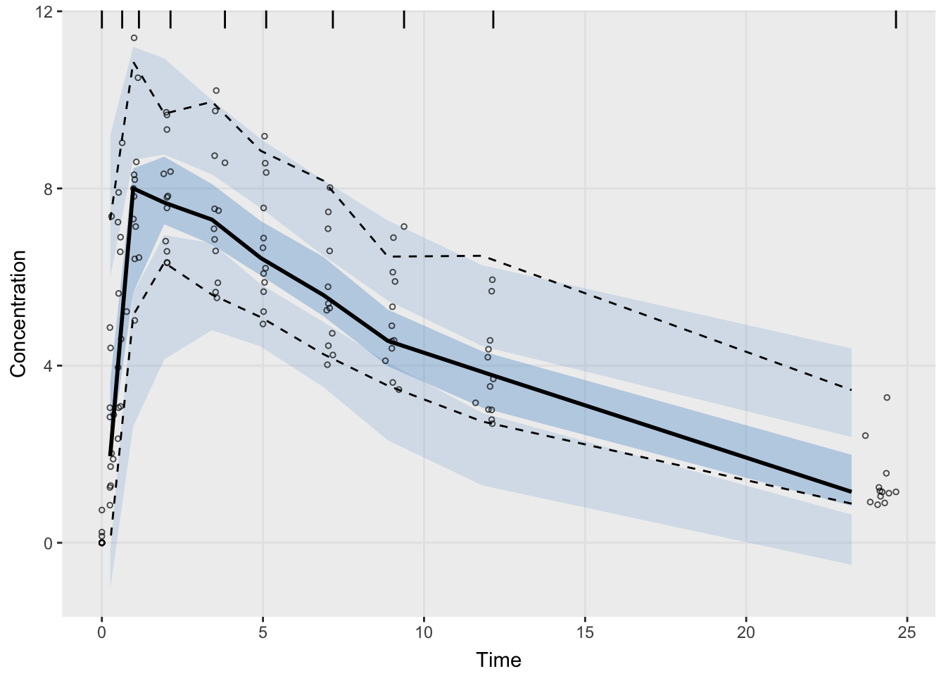
A common way to create Visual Predictive Checks in nlmixr2plot is the vpcPlot() function.
The function automates the simulation, interval calculation, and plotting steps needed to generate a VPC.
vpcPlot(
  fit,
  n = 100,
  show = list(
    obs_dv = TRUE
  ),
  bins = "jenks",
  xlab = "Time",
  ylab = "Concentration"
)
Explanation of key arguments:
n = 100
Number of simulated studies

show = list(obs_dv = TRUE)
Display observed concentrations

bins = "jenks"
Automatically choose time bins
Interpretation:
A VPC typically displays:
- observed data (points or summaries)
- simulated prediction intervals
- uncertainty around simulated behavior
Conceptually:
Observed Data
↓
Simulate New Studies
↓
Compute Prediction Intervals
↓
Compare Observed vs Simulated
When interpreting the VPC, ask:
- Do observations mostly stay inside simulated intervals?
- Does the overall trend match simulations?
- Does variability appear similar?
Small deviations are expected.
We are looking for overall agreement, not perfect overlap.
Optional: Increase Simulation Replicates
Simulation count affects smoothness.
Example:
vpcPlot(
  fit,
  n = 500
)
Interpretation:
More Simulations
↓
Smoother Prediction Intervals
Higher values improve stability but increase runtime.
Worked Example 2: What Good Agreement Looks Like
Look for:
- observed median tracking simulated median
- observations remaining mostly inside prediction intervals
- similar variability across time
Small local deviations are acceptable.
Focus on overall agreement.
Worked Example 3: Recognize Warning Signs
Possible concerns:
Observed Above Band
↓
Underprediction

Observed Below Band
↓
Overprediction

Observed Variability Wider
↓
Variability Underestimated
Patterns matter more than isolated observations.
Worked Example 4: Diagnostic Workflow
Structure

↓

Variability

↓

Covariates

↓

GOF

↓

Residuals

↓

VPC

↓

Qualification
VPC evaluates the entire model.
Strategies
- inspect central tendency
- inspect variability
- avoid focusing on single points
Common Mistakes
- expecting perfect overlap
- diagnosing from isolated observations
- treating VPC as the only diagnostic
Practice Problems
What question does a VPC answer?
Why is simulation required?
Generate:
vpcPlot(
  fit,
  n = 100,
  show = list(
    obs_dv = TRUE
  ),
  bins = "jenks",
  xlab = "Time",
  ylab = "Concentration"
)
Describe one observation.
- What could observations consistently above the upper interval suggest?
- structure?
- variability?
- covariates?
- residual assumptions?
- Why should VPC be interpreted together with GOF and residual diagnostics?
TipStep-by-Step Solutions
Problem 1
A VPC asks:
If the fitted model were true, would data like ours commonly occur?
Unlike GOF plots, VPC evaluates both prediction and variability.
Problem 2
Simulation is required because a single prediction cannot describe variability.
The model repeatedly generates new datasets and compares them with observations.
Problem 3
Generate:
vpcPlot(
  fit,
  n = 100,
  show = list(
    obs_dv = TRUE
  ),
  bins = "jenks",
  xlab = "Time",
  ylab = "Concentration"
)
Inspect:
- overall trend
- simulated intervals
- spread
Ask:
Do observations behave similarly to simulations?Problem 4
Observations consistently above the upper interval may suggest:
Model predicts too low
↓
Underprediction
Problem 5
Each diagnostic answers a different question:
GOF
Prediction quality

Residuals
Bias and trends

VPC
Variability reproduction
Model qualification combines all three.
Summary
- VPC evaluates prediction and variability
- simulations evaluate the full model
- VPC complements GOF and residual diagnostics
- diagnostics should be interpreted collectively
TipQuick Tips
- Simulate before concluding
- Variability matters
- Use multiple diagnostics