Loading and Exploring the Course Dataset

Load the theo_sd dataset from nlmixr2data and inspect its structure before modeling.

Tip

Big picture: Before fitting a model, we need to know what the dataset contains, what each row represents, and whether the event records make sense.

Learning Objectives

By the end of this lesson, you will be able to:

Load the course dataset from the nlmixr2data package.
Inspect the structure of an event-based PK dataset.
Identify dosing and observation records.
Count subjects, observations, and dose records.
Interpret key columns such as ID, TIME, DV, AMT, and EVID.
Prepare for subject-level exploratory visualization.

Key Ideas

theo_sd is the main teaching dataset for the early PopPK modules.
The dataset is already organized in an event-based format.
Dosing records and observation records are stored together.
Observation records usually have EVID == 0.
Dose records usually have EVID == 1.
Inspecting structure comes before plotting or modeling.

Why We Use `theo_sd`

The theophylline dataset is a classic PK teaching dataset. In this course, we use theo_sd from the nlmixr2data package because it is already organized for population modeling workflows.

This lets us work directly with columns commonly used by population modeling software, including:

ID
TIME
DV
AMT
EVID

Note

Not every pharmacometric dataset contains the same variables.

For example, theo_sd uses EVID to distinguish dosing and observation records and does not include an explicit MDV column.

Additional modeling variables exist, but they are not required to understand the concepts in this lesson and will be introduced later when needed.

Setup

library(tidyverse)
library(nlmixr2data)

Load the dataset:

data("theo_sd", package = "nlmixr2data")

Create a local working copy:

theo <- theo_sd

Worked Example 1: Inspect the Dataset

Start by looking at the object structure.

glimpse(theo)

Rows: 144
Columns: 7
$ ID   <int> 1, 1, 1, 1, 1, 1, 1, 1, 1, 1, 1, 1, 2, 2, 2, 2, 2, 2, 2, 2, 2, 2,…
$ TIME <dbl> 0.00, 0.00, 0.25, 0.57, 1.12, 2.02, 3.82, 5.10, 7.03, 9.05, 12.12…
$ DV   <dbl> 0.00, 0.74, 2.84, 6.57, 10.50, 9.66, 8.58, 8.36, 7.47, 6.89, 5.94…
$ AMT  <dbl> 319.992, 0.000, 0.000, 0.000, 0.000, 0.000, 0.000, 0.000, 0.000, …
$ EVID <int> 101, 0, 0, 0, 0, 0, 0, 0, 0, 0, 0, 0, 101, 0, 0, 0, 0, 0, 0, 0, 0…
$ CMT  <int> 1, 2, 2, 2, 2, 2, 2, 2, 2, 2, 2, 2, 1, 2, 2, 2, 2, 2, 2, 2, 2, 2,…
$ WT   <dbl> 79.6, 79.6, 79.6, 79.6, 79.6, 79.6, 79.6, 79.6, 79.6, 79.6, 79.6,…

View the first rows:

theo %>% slice_head(n = 10)

   ID TIME    DV     AMT EVID CMT   WT
1   1 0.00  0.00 319.992  101   1 79.6
2   1 0.00  0.74   0.000    0   2 79.6
3   1 0.25  2.84   0.000    0   2 79.6
4   1 0.57  6.57   0.000    0   2 79.6
5   1 1.12 10.50   0.000    0   2 79.6
6   1 2.02  9.66   0.000    0   2 79.6
7   1 3.82  8.58   0.000    0   2 79.6
8   1 5.10  8.36   0.000    0   2 79.6
9   1 7.03  7.47   0.000    0   2 79.6
10  1 9.05  6.89   0.000    0   2 79.6

At this stage, do not try to model anything yet. The goal is simply to understand what is in the dataset.

Dataset Dimensions

How many rows and columns are present?

dim(theo)

[1] 144   7

A useful readable summary:

tibble(
  n_rows = nrow(theo),
  n_columns = ncol(theo)
)

# A tibble: 1 × 2
  n_rows n_columns
   <int>     <int>
1    144         7

Worked Example 2: Count Subjects and Events

Count the number of unique subjects.

theo %>%
  summarise(
    n_subjects = n_distinct(ID)
  )

  n_subjects
1         12

Count rows by event type.

theo %>%
  count(EVID)

  EVID   n
1    0 132
2  101  12

Interpretation:

EVID == 0 usually indicates observation rows.
Nonzero EVID values indicate dosing or other event records.
In theo_sd, dosing records use EVID == 101, which encodes a dose event into a specific compartment.

Observation and Dose Records

Create separate objects for observations and doses.

obs <- theo %>%
  filter(EVID == 0)

dose <- theo %>%
  filter(EVID != 0)

Check their sizes.

tibble(
  n_observation_rows = nrow(obs),
  n_dose_rows = nrow(dose)
)

# A tibble: 1 × 2
  n_observation_rows n_dose_rows
               <int>       <int>
1                132          12

This separation is useful for summaries, QC, and visualization.

Worked Example 3: Inspect Observation Records

Observation records contain measured concentrations.

obs %>%
  select(ID, TIME, DV, AMT, EVID) %>%
  slice_head(n = 10)

   ID  TIME    DV AMT EVID
1   1  0.00  0.74   0    0
2   1  0.25  2.84   0    0
3   1  0.57  6.57   0    0
4   1  1.12 10.50   0    0
5   1  2.02  9.66   0    0
6   1  3.82  8.58   0    0
7   1  5.10  8.36   0    0
8   1  7.03  7.47   0    0
9   1  9.05  6.89   0    0
10  1 12.12  5.94   0    0

Check whether observation rows have concentration values.

obs %>%
  summarise(
    n_obs = n(),
    n_missing_dv = sum(is.na(DV)),
    n_nonmissing_dv = sum(!is.na(DV))
  )

  n_obs n_missing_dv n_nonmissing_dv
1   132            0             132

Worked Example 4: Inspect Dose Records

Dose records describe when drug entered the system.

dose %>%
  select(ID, TIME, AMT, DV, EVID) %>%
  slice_head(n = 10)

   ID TIME     AMT DV EVID
1   1    0 319.992  0  101
2   2    0 318.560  0  101
3   3    0 319.365  0  101
4   4    0 319.880  0  101
5   5    0 319.956  0  101
6   6    0 320.000  0  101
7   7    0 319.770  0  101
8   8    0 319.365  0  101
9   9    0 267.840  0  101
10 10    0 320.100  0  101

Summarize dose amounts.

dose %>%
  count(AMT)

       AMT n
1  267.840 1
2  318.560 1
3  319.365 2
4  319.770 1
5  319.800 1
6  319.880 1
7  319.956 1
8  319.992 1
9  320.000 1
10 320.100 1
11 320.650 1

For many simple PK examples, each subject receives one dose at time zero. We should still verify that assumption rather than assume it.

Time Range

Check the time range in the full dataset.

theo %>%
  summarise(
    min_time = min(TIME, na.rm = TRUE),
    max_time = max(TIME, na.rm = TRUE)
  )

  min_time max_time
1        0    24.65

Check the observation-time range.

obs %>%
  summarise(
    min_obs_time = min(TIME, na.rm = TRUE),
    max_obs_time = max(TIME, na.rm = TRUE)
  )

  min_obs_time max_obs_time
1            0        24.65

Worked Example 5: Subject-Level Summary

Before plotting profiles, summarize how many observations each subject has.

obs_by_id <- obs %>%
  count(ID, name = "n_obs") %>%
  arrange(ID)

obs_by_id

   ID n_obs
1   1    11
2   2    11
3   3    11
4   4    11
5   5    11
6   6    11
7   7    11
8   8    11
9   9    11
10 10    11
11 11    11
12 12    11

Check whether subjects have the same number of observations.

obs_by_id %>%
  count(n_obs)

  n_obs  n
1    11 12

This helps us understand whether the dataset is balanced or unbalanced.

Initial Subject-Level Characteristics

Before modeling, it is often useful to inspect subject-level variables that may later become candidate covariates.

For example, theo_sd contains body weight (WT).

At this stage, we are not testing covariate effects. We are simply understanding the study population.

Summarize weight:

theo %>%
  distinct(ID, WT) %>%
  summarise(
    n_subjects = n(),
    wt_min = min(WT, na.rm = TRUE),
    wt_median = median(WT, na.rm = TRUE),
    wt_max = max(WT, na.rm = TRUE)
  )

  n_subjects wt_min wt_median wt_max
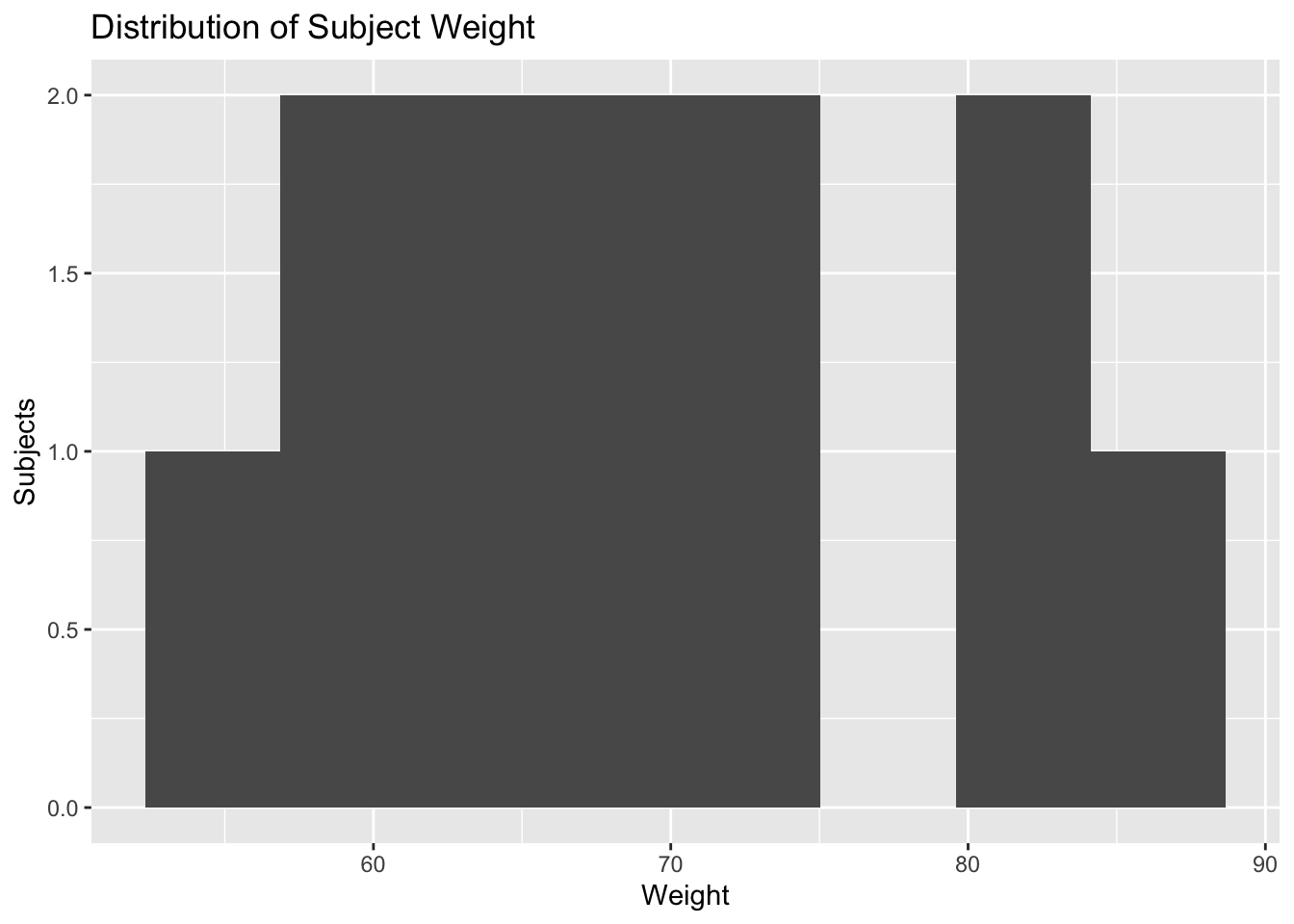
1         12   54.6      70.5   86.4

Visualize weight distribution:

theo %>%
  distinct(ID, WT) %>%
  ggplot(aes(WT)) +
  geom_histogram(bins = 8) +
  labs(
    title = "Distribution of Subject Weight",
    x = "Weight",
    y = "Subjects"
  )

At this stage, the goal is not interpretation of weight effects.

Instead, the goal is to ask:

Is the population homogeneous?
Is there meaningful variability?
Could this variable become important later?

Covariate relationships will be introduced formally in a later module.

Quick First Look at Profiles

A small plot can help verify that the data behave like PK concentration-time data.

ggplot(obs, aes(TIME, DV, group = ID)) +
  geom_line(alpha = 0.35) +
  geom_point(size = 0.8) +
  labs(
    title = "Observed Theophylline Concentration-Time Profiles",
    x = "Time",
    y = "Concentration"
  )

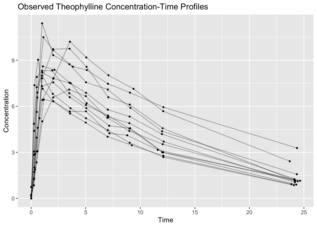
We will build more intentional exploratory plots in a later lesson.

Strategies

Start with glimpse().
Count subjects and event types.
Separate observation and dosing records.
Check missing values in DV.
Verify the dose amounts and dose times.
Summarize observations by subject before plotting.

Common Mistakes

Using all rows when plotting observed concentrations.
Forgetting to filter EVID == 0 for observation summaries.
Assuming AMT == 0 means the row is unimportant.
Treating the dataset as a simple spreadsheet rather than an event history.

Practice Problems

Count the number of subjects in theo.
Count the number of observation rows and dose rows.
Find the minimum and maximum observed concentration.
Count the number of observations per subject.
Create a simple concentration-time plot using only observation rows.

Step-by-Step Solutions

Problem 1: Count the number of subjects

theo %>%
  summarise(n_subjects = n_distinct(ID))

  n_subjects
1         12

Problem 2: Count observation and dose rows

theo %>%
  count(EVID)

  EVID   n
1    0 132
2  101  12

Problem 3: Find the minimum and maximum observed concentration

obs %>%
  summarise(
    min_dv = min(DV, na.rm = TRUE),
    max_dv = max(DV, na.rm = TRUE)
  )

  min_dv max_dv
1      0   11.4

Problem 4: Count observations per subject

obs %>%
  count(ID, name = "n_obs") %>%
  arrange(ID)

   ID n_obs
1   1    11
2   2    11
3   3    11
4   4    11
5   5    11
6   6    11
7   7    11
8   8    11
9   9    11
10 10    11
11 11    11
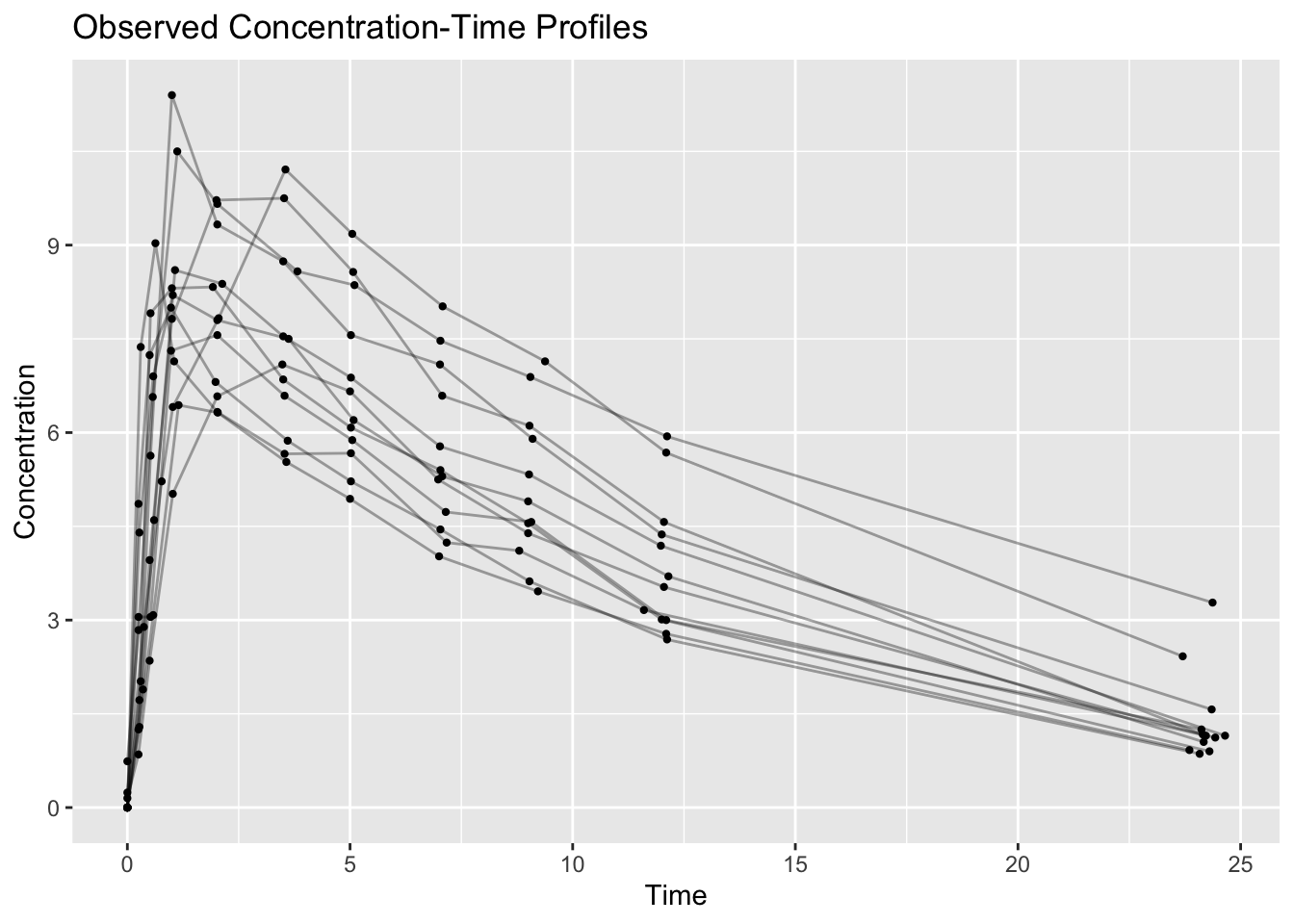
12 12    11

Problem 5: Create a simple concentration-time plot

ggplot(obs, aes(TIME, DV, group = ID)) +
  geom_line(alpha = 0.35) +
  geom_point(size = 0.8) +
  labs(
    title = "Observed Concentration-Time Profiles",
    x = "Time",
    y = "Concentration"
  )

Summary

You loaded theo_sd from nlmixr2data.
You inspected the dataset structure.
You separated observation and dose records.
You summarized subjects, events, dose amounts, and observation times.
You created a first simple concentration-time plot.

Quick Tips

Use EVID == 0 for observed concentration summaries.
Check dose records before modeling.
Count first, plot second, model later.
Treat the dataset as a sequence of events over time.

Learning Objectives

Key Ideas

Why We Use theo_sd

Setup

Worked Example 1: Inspect the Dataset

Dataset Dimensions

Worked Example 2: Count Subjects and Events

Observation and Dose Records

Worked Example 3: Inspect Observation Records

Worked Example 4: Inspect Dose Records

Time Range

Worked Example 5: Subject-Level Summary

Initial Subject-Level Characteristics

Quick First Look at Profiles

Strategies

Common Mistakes

Practice Problems

Summary

Why We Use `theo_sd`