library(tidyverse)
library(nlmixr2data)

data("theo_sd", package = "nlmixr2data")

theo <- theo_sd

obs <- theo %>%
  filter(EVID == 0)

dose <- theo %>%
filter(EVID != 0)Preparing Analysis-Ready Data
Perform modeling-focused quality checks and prepare a clean working dataset before visualization and model building.
Tip
Big picture: Population modeling starts long before estimation. Before fitting models, we should confirm that the dataset structure, event records, and observations make scientific sense.
Learning Objectives
By the end of this lesson, you will be able to:
- Perform modeling-focused QC checks.
- Verify event records and observations.
- Interpret missingness in event-based datasets.
- Check dose and observation consistency.
- Create a clean modeling object for later lessons.
Key Ideas
- QC is part of modeling.
- Missing values should be interpreted in context.
- Event structure should be verified before estimation.
- Modeling objects should be reproducible.
- Data understanding comes before visualization.
Setup
Why Data Preparation Matters
Modeling assumes that the dataset reflects what happened in the study.
Before fitting models, ask:
- Are observations present?
- Are event records sensible?
- Are times ordered?
- Are dose amounts reasonable?
- Do subject summaries look plausible?
Many apparent modeling failures are actually data problems.
Worked Example 1: Interpret Missing Values
missing_summary <- theo %>%
  summarise(
    across(
      everything(),
      ~sum(is.na(.))
    )
  ) %>%
  pivot_longer(
    everything(),
    names_to = "variable",
    values_to = "n_missing"
  ) %>%
  arrange(desc(n_missing))

missing_summary
# A tibble: 7 × 2
variable n_missing
<chr> <int>
1 ID 0
2 TIME 0
3 DV 0
4 AMT 0
5 EVID 0
6 CMT 0
7 WT 0Interpretation:
- dose rows may not contain observations
- observation rows may not contain dose amounts
Missing values are not automatically errors.
Worked Example 2: Verify Event Consistency
theo %>%
  count(EVID)
EVID n
1 0 132
2 101 12Interpretation:
EVID == 0→ observation rows- nonzero
EVID→ event rows
Check ordering:
event_order <- theo %>%
  group_by(ID) %>%
  summarise(
    ordered = all(diff(TIME) >= 0),
    .groups = "drop"
  )

event_order
# A tibble: 12 × 2
ID ordered
<int> <lgl>
1 1 TRUE
2 2 TRUE
3 3 TRUE
4 4 TRUE
5 5 TRUE
6 6 TRUE
7 7 TRUE
8 8 TRUE
9 9 TRUE
10 10 TRUE
11 11 TRUE
12 12 TRUE Review failures:
event_order %>%
  filter(!ordered)
# A tibble: 0 × 2
# ℹ 2 variables: ID <int>, ordered <lgl>Worked Example 3: Verify Dose Records
dose %>%
  summarise(
    n_dose_rows = n(),
    n_unique_doses = n_distinct(AMT),
    dose_min = min(AMT, na.rm = TRUE),
    dose_max = max(AMT, na.rm = TRUE)
  )
n_dose_rows n_unique_doses dose_min dose_max
1 12 11 267.84 320.65Review values:
dose %>%
  count(AMT)
AMT n
1 267.840 1
2 318.560 1
3 319.365 2
4 319.770 1
5 319.800 1
6 319.880 1
7 319.956 1
8 319.992 1
9 320.000 1
10 320.100 1
11 320.650 1At this stage, we are verifying assumptions—not modeling dose effects.
Worked Example 4: Observation QC
obs %>%
  summarise(
    min_dv = min(DV, na.rm = TRUE),
    median_dv = median(DV, na.rm = TRUE),
    max_dv = max(DV, na.rm = TRUE)
  )
min_dv median_dv max_dv
1 0 5.275 11.4Observation counts:
obs %>%
  count(ID, name = "n_obs")
ID n_obs
1 1 11
2 2 11
3 3 11
4 4 11
5 5 11
6 6 11
7 7 11
8 8 11
9 9 11
10 10 11
11 11 11
12 12 11Subject-Level QC
Inspect variables that may later become covariates.
theo %>%
  distinct(ID, WT) %>%
  summarise(
    wt_min = min(WT, na.rm = TRUE),
    wt_median = median(WT, na.rm = TRUE),
    wt_max = max(WT, na.rm = TRUE)
  )
wt_min wt_median wt_max
1 54.6 70.5 86.4Visualize:
theo %>%
  distinct(ID, WT) %>%
  ggplot(aes(WT)) +
  geom_histogram(bins = 8) +
  labs(
    title = "Distribution of Subject Weight",
    x = "Weight",
    y = "Subjects"
  )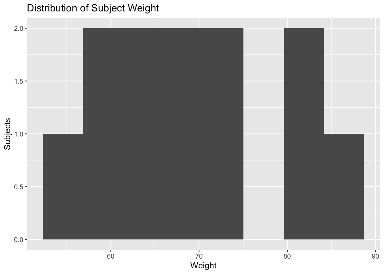
At this stage, we are describing covariates—not modeling them.
Worked Example 5: Create a Modeling Object
theo_model <- theo %>%
  arrange(ID, TIME)
Check dimensions:
dim(theo_model)[1] 144 7At this stage:
- no rows are removed
- no values are changed
- no transformations are applied
The goal is simply to establish a reviewed dataset object.
QC Checklist
- event records reviewed
- observations inspected
- dose assumptions checked
- missing values interpreted
- subject summaries reviewed
- modeling object created
Strategies
- Count before plotting.
- Separate observations and event records.
- Verify assumptions explicitly.
- Keep a clean working object.
Common Mistakes
- Deleting rows without justification.
- Assuming datasets are modeling-ready.
- Treating QC as optional.
- Confusing cleaning with modeling.
Practice Problems
- Summarize missing values.
- Count event types.
- Summarize dose values.
- Count observations per subject.
- Create a reviewed modeling object.
TipStep-by-Step Solutions
Use the QC examples in this lesson and interpret outputs before moving on.
Focus on understanding the data—not changing it.
Summary
- Modeling begins with QC.
- Event records should be validated.
- Missing values require context.
- Subject characteristics provide modeling context.
- Create clean modeling objects before moving forward.
TipQuick Tips
- Inspect first.
- Model second.
- Verify assumptions.
- Keep reviewed working objects.