library(tidyverse)
library(nlmixr2)
library(nlmixr2data)

data("theo_sd", package = "nlmixr2data")Reading the Fit Object
Explore the nlmixr2 fit object and understand the main components returned after estimation.
Tip
Big picture: Model fitting produces much more than parameter estimates. The fit object stores model structure, parameter estimates, uncertainty information, predictions, residuals, variability estimates, and metadata.
Learning Objectives
By the end of this lesson, you will be able to:
- Understand what the fit object contains.
- View the estimated model structure.
- Read the printed fit summary.
- Locate parameter estimates and uncertainty information.
- Extract predictions and residual variables.
- Recognize which outputs belong to estimation versus later diagnostics.
Key Ideas
- Estimation returns a rich fit object.
fitandprint(fit)display different useful views.- The fit object contains more than coefficients.
- Model output should be read systematically.
- Fit interpretation comes before diagnostics.
Setup
Fit the model.
one_comp_model <- function(){

  ini({

    tka <- log(1)
    tcl <- log(3)
    tv  <- log(30)

    eta.ka ~ 0.1
    eta.cl ~ 0.1
    eta.v  ~ 0.1

    add.err <- 0.1

  })

  model({

    ka <- exp(tka + eta.ka)
    cl <- exp(tcl + eta.cl)
    v  <- exp(tv + eta.v)

    linCmt() ~ add(add.err)

  })

}

fit <-
nlmixr2(
  one_comp_model,
  theo_sd,
  est = "focei",
  control = list(
    print = 0
  )
)
Why the Fit Object Matters
After estimation, the model becomes more than equations.
The fit object contains:
Model
+
Data
+
Estimated Parameters
+
Predictions
+
Residuals
+
Variability
+
Metadata
Understanding this structure helps us move from model fitting to model interpretation.
Worked Example 1: View the Estimated Model
Start by viewing the fitted model.
fit\[\begin{align*} {ka} & = \exp\left({tka}+{eta.ka}\right) \\ {cl} & = \exp\left({tcl}+{eta.cl}\right) \\ {v} & = \exp\left({tv}+{eta.v}\right) \\ linCmt() & \sim add({add.err}) \end{align*}\]
This renders a useful model representation.
This view helps connect:
Structural Model
↓
Population Parameters
↓
Subject Variability
↓
Observation Model
Look for:
- model equations
- parameter names
- variability terms
- residual error structure
At this stage, focus on recognizing the model.
Detailed numerical interpretation comes next.
Worked Example 2: Print the Fit Summary
Print the complete fit summary.
print(fit)── nlmixr² FOCEi (outer: nlminb) ──
OBJF AIC BIC Log-likelihood Condition#(Cov) Condition#(Cor)
FOCEi 116.8039 373.4036 393.5832 -179.7018 68.64196 9.387133
── Time (sec $time): ──
setup optimize covariance table other
elapsed 0.001914 0.145002 0.145003 0.022 3.339081
── Population Parameters ($parFixed or $parFixedDf): ──
Est. SE %RSE Back-transformed(95%CI) BSV(CV%) Shrink(SD)%
tka 0.463 0.195 42.1 1.59 (1.08, 2.33) 70.5 1.86%
tcl 1.01 0.0751 7.42 2.75 (2.37, 3.19) 26.8 3.98%
tv 3.46 0.0436 1.26 31.8 (29.2, 34.6) 13.9 10.4%
add.err 0.694 0.694
Covariance Type ($covMethod): r,s
No correlations in between subject variability (BSV) matrix
Full BSV covariance ($omega) or correlation ($omegaR; diagonals=SDs)
Distribution stats (mean/skewness/kurtosis/p-value) available in $shrink
Information about run found ($runInfo):
• gradient problems with initial estimate and covariance; see $scaleInfo
• ETAs were reset to zero during optimization; (Can control by foceiControl(resetEtaP=.))
• initial ETAs were nudged; (can control by foceiControl(etaNudge=., etaNudge2=))
Censoring ($censInformation): No censoring
Minimization message ($message):
relative convergence (4)
── Fit Data (object is a modified tibble): ──
# A tibble: 132 × 22
ID TIME DV PRED RES WRES IPRED IRES IWRES CPRED CRES CWRES
<fct> <dbl> <dbl> <dbl> <dbl> <dbl> <dbl> <dbl> <dbl> <dbl> <dbl> <dbl>
1 1 0 0.74 0 0.74 1.07 0 0.74 1.07 0 0.74 1.07
2 1 0.25 2.84 3.26 -0.422 -0.225 3.85 -1.01 -1.45 3.22 -0.378 -0.177
3 1 0.57 6.57 5.83 0.740 0.297 6.78 -0.215 -0.310 5.77 0.796 0.287
# ℹ 129 more rows
# ℹ 10 more variables: eta.ka <dbl>, eta.cl <dbl>, eta.v <dbl>, depot <dbl>,
# central <dbl>, ka <dbl>, cl <dbl>, v <dbl>, tad <dbl>, dosenum <dbl>The printed summary contains several sections.
Focus on these first.
Objective Function
Inspect:
OBJFThe objective function is the quantity minimized during estimation.
Conceptually:
Model Parameters

↓

Generate Predictions

↓

Compare to Observations

↓

Calculate Likelihood

↓

Convert to Objective Function
nlmixr2 estimates parameters by searching for values that improve agreement between observed and predicted data.
In general:
Higher Likelihood

↓

Lower Objective Function
Lower objective function values may suggest better agreement for the same dataset and model structure.
Do not compare objective function values across unrelated datasets or substantially different analyses.
Information Criteria
Inspect:
AIC
BIC
These balance:
Model Fit
↓
Model Complexity
Lower values may indicate a more efficient model.
These become more useful later when comparing candidate models.
Population Parameters
Inspect:
Est.
SE
%RSE
Back-transformed
Interpretation:
Est.→ estimated value on the model scaleSE→ standard error%RSE→ relative standard errorBack-transformed→ estimate on the original PK scale
Variability
Inspect:
BSV(CV%)This estimates subject-to-subject variability.
The next module explains variability models in more detail.
Shrinkage
Inspect:
Shrink(SD)%Shrinkage gives information about how strongly individual estimates are informed by the data.
At this stage, do not apply strict thresholds.
Just recognize where shrinkage appears.
Convergence
Inspect:
fit$messageExample:
relative convergence (4)Interpretation:
Convergence means optimization stopped successfully.
This does not guarantee:
- biologically reasonable estimates
- realistic variability
- predictive performance
Those questions are addressed later in the course.
Worked Example 3: Explore the Object Structure
Inspect the fit object class.
class(fit)[1] "nlmixr2FitData" "nlmixr2FitCore" "nlmixr2.focei" "tbl_df"
[5] "tbl" "data.frame"
attr(,".foceiEnv")Explore available components.
names(fit) [1] "ID" "TIME" "DV" "PRED" "RES" "WRES" "IPRED"
[8] "IRES" "IWRES" "CPRED" "CRES" "CWRES" "eta.ka" "eta.cl"
[15] "eta.v" "depot" "central" "ka" "cl" "v" "tad"
[22] "dosenum"This gives a quick overview of what is stored.
The goal is not to memorize every component.
The goal is to learn how to navigate the object.
Worked Example 4: Extract Population Parameters
Extract fixed effects.
coef(fit)$fixed %>%
  enframe(
    name = "parameter",
    value = "estimate"
  )
# A tibble: 4 × 2
parameter estimate
<chr> <dbl>
1 tka 0.463
2 tcl 1.01
3 tv 3.46
4 add.err 0.694These estimates are on the model scale.
Convert them to the original scale.
coef(fit)$fixed %>%
exp() %>%
enframe(
  name = "parameter",
  value = "estimate_original_scale"
)
# A tibble: 4 × 2
parameter estimate_original_scale
<chr> <dbl>
1 tka 1.59
2 tcl 2.75
3 tv 31.8
4 add.err 2.00Interpretation:
tka→ typical absorptiontcl→ typical clearancetv→ typical volume
These values describe the typical subject.
Worked Example 5: Inspect Predictions and Residual Variables
Extract fitted output.
fit_tbl <-
fit %>%
as_tibble()

fit_tbl
# A tibble: 132 × 22
ID TIME DV PRED RES WRES IPRED IRES IWRES CPRED CRES
<fct> <dbl> <dbl> <dbl> <dbl> <dbl> <dbl> <dbl> <dbl> <dbl> <dbl>
1 1 0 0.74 0 0.74 1.07 0 0.74 1.07 0 0.74
2 1 0.25 2.84 3.26 -0.422 -0.225 3.85 -1.01 -1.45 3.22 -0.378
3 1 0.57 6.57 5.83 0.740 0.297 6.78 -0.215 -0.310 5.77 0.796
4 1 1.12 10.5 7.87 2.63 1.23 9.04 1.46 2.10 7.83 2.67
5 1 2.02 9.66 8.51 1.15 0.826 9.79 -0.125 -0.180 8.49 1.17
6 1 3.82 8.58 7.62 0.955 0.805 9.09 -0.514 -0.741 7.62 0.957
7 1 5.1 8.36 6.84 1.52 1.30 8.45 -0.0853 -0.123 6.84 1.52
8 1 7.03 7.47 5.79 1.68 1.44 7.54 -0.0682 -0.0983 5.78 1.69
9 1 9.05 6.89 4.87 2.02 1.70 6.69 0.198 0.286 4.83 2.06
10 1 12.1 5.94 3.73 2.21 1.84 5.58 0.356 0.514 3.64 2.30
# ℹ 122 more rows
# ℹ 11 more variables: CWRES <dbl>, eta.ka <dbl>, eta.cl <dbl>, eta.v <dbl>,
# depot <dbl>, central <dbl>, ka <dbl>, cl <dbl>, v <dbl>, tad <dbl>,
# dosenum <dbl>View available variables.
names(fit_tbl) [1] "ID" "TIME" "DV" "PRED" "RES" "WRES" "IPRED"
[8] "IRES" "IWRES" "CPRED" "CRES" "CWRES" "eta.ka" "eta.cl"
[15] "eta.v" "depot" "central" "ka" "cl" "v" "tad"
[22] "dosenum"Common variables include:
| Variable | Meaning |
|---|---|
DV |
observed concentration |
PRED |
prediction for the typical subject |
IPRED |
prediction including individual effects |
RES |
observed − population prediction |
IRES |
observed − individual prediction |
CWRES |
conditional weighted residual |
These quantities become central for:
- understanding model behavior
- variability interpretation
- later diagnostic evaluation
For now, recognize that the fit object stores them automatically.
Worked Example 6: Create a First Prediction Plot
Create a simple observed versus population prediction plot.
ggplot(
  fit_tbl,
  aes(PRED, DV)
) +
geom_point(
  alpha = 0.35
) +
geom_abline(
  slope = 1,
  intercept = 0,
  linetype = 2
) +
labs(
  title = "Observed vs Population Prediction",
  x = "PRED",
  y = "DV"
)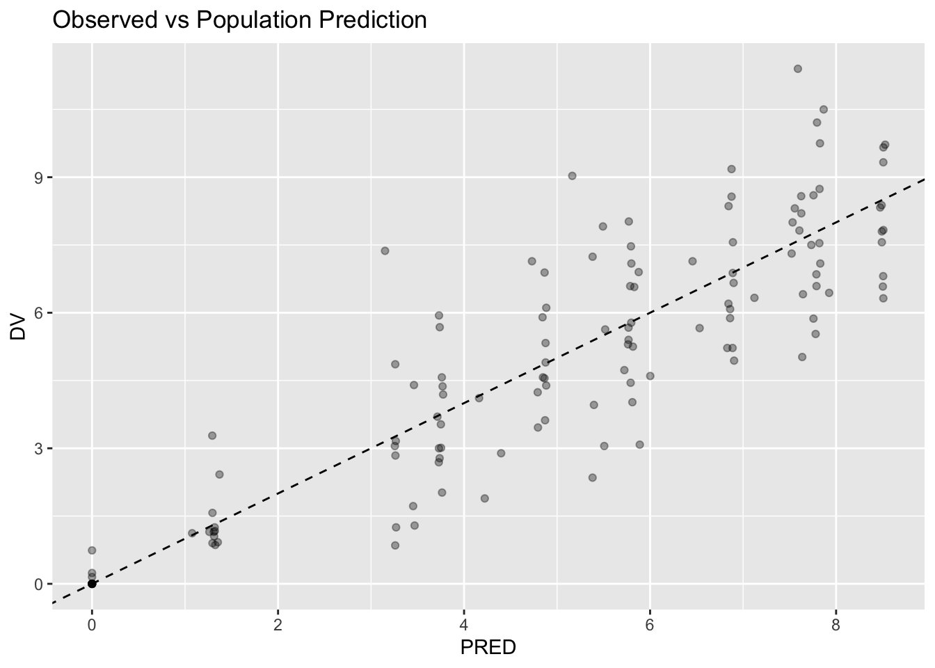
Interpretation:
- points closer to the line suggest stronger agreement
- scatter is expected
- formal diagnostics come later
This plot is only a preview.
Do not use it alone to judge model adequacy.
Reading Output Systematically
Suggested order:
Model Representation
↓
Fit Summary
↓
Convergence
↓
Parameter Estimates
↓
Variability
↓
Predictions
↓
Diagnostics
Avoid reading everything simultaneously.
Strategies
- Start with the model structure.
- Read the printed summary next.
- Extract specific quantities directly.
- Interpret estimates on the correct scale.
- Save full diagnostic interpretation for the diagnostics module.
Common Mistakes
- Treating output as final truth.
- Confusing predictions and observations.
- Forgetting that log-scale parameters need back-transformation.
- Skipping fit inspection.
- Assuming convergence means the model is adequate.
Practice Problems
What is the difference between running
fitandprint(fit)in this lesson?What types of information are stored inside
fit?Run:
print(fit)Identify:
- one uncertainty metric
- one variability metric
- one convergence message
- Extract fixed effects.
coef(fit)$fixed %>%
enframe(
  name = "parameter",
  value = "estimate"
)
Then back-transform them.
coef(fit)$fixed %>%
exp() %>%
enframe(
  name = "parameter",
  value = "estimate_original_scale"
)
Why is the second table easier to interpret biologically?
- Inspect prediction variables.
fit_tbl %>%
select(
  DV,
  PRED,
  IPRED,
  RES,
  CWRES
) %>%
head()
Explain in words how DV, PRED, IPRED, RES, and CWRES differ.
TipStep-by-Step Solutions
Problem 1
Running:
fitrenders a visual model representation in Quarto.
This is useful for seeing:
- model equations
- parameter relationships
- residual error structure
Running:
print(fit)prints the full fit summary.
This is useful for seeing:
- objective function
- information criteria
- parameter estimates
- uncertainty metrics
- variability estimates
- convergence information
Problem 2
fit stores more than parameter estimates.
Examples include:
- model structure
- fixed effects
- variability estimates
- predictions
- residual quantities
- estimation metadata
The fit object becomes the central object for later analysis.
Problem 3
In the printed summary, examples include:
SE
↓
parameter uncertainty
%RSE
↓
relative parameter uncertaintyBSV(CV%)
↓
subject-to-subject variabilityrelative convergence
↓
optimization statusThe goal is to learn where information appears, not to memorize every line.
Problem 4
The first table shows estimates on the model scale.
For example:
tcl
=
log(CL)
The second table uses:
exp()to return estimates to the original scale.
This is easier to interpret biologically because clearance, volume, and absorption are positive PK parameters.
Problem 5
Example interpretation:
| Variable | Meaning |
|---|---|
DV |
observed concentration |
PRED |
prediction for the typical subject |
IPRED |
prediction including individual effects |
RES |
observed minus population prediction |
CWRES |
standardized residual used for diagnostics |
Conceptually:
DV
Observed Data

PRED
Typical Subject Prediction

IPRED
Subject-Specific Prediction

RES
Raw Disagreement

CWRES
Standardized Diagnostic Residual
These variables become central later when evaluating model behavior.
Summary
- Estimation returns a rich fit object.
fitrenders the model representation in Quarto.print(fit)prints the full fit summary.- Fit objects contain estimates, uncertainty metrics, predictions, residuals, and metadata.
- Systematic reading improves interpretation.
TipQuick Tips
- Use
fitto view the model. - Use
print(fit)to inspect the summary. - Extract before interpreting.
- Back-transform log-scale parameters.
- Diagnostics come later.