library(tidyverse)What Is a Structural PK Model?
Understand structural PK models as the expected biological pattern behind concentration-time data.
Tip
Big picture: A structural PK model describes the expected concentration-time pattern after dosing before we add variability, residual error, or covariates.
Learning Objectives
By the end of this lesson, you will be able to:
- Explain what a structural PK model represents.
- Distinguish structural behavior from variability.
- Describe how dose, absorption, distribution, and elimination shape concentration-time profiles.
- Recognize why structural models come before population models.
- Connect observed PK profiles to candidate model assumptions.
Key Ideas
- Structural models describe expected biological behavior.
- Structural PK models translate dosing history into concentration-time predictions.
- Variability is added later; the structural model is the starting point.
- The same structural model can be used for simulation and estimation.
- Good structural thinking makes later diagnostics easier to interpret.
Setup
Why Structural Models Matter
In the previous Module, we inspected the dataset and visualized concentration-time profiles.
Now we ask a new question:
What type of mathematical structure could generate these profiles?
A structural PK model represents the expected concentration-time behavior after dosing.
It describes processes such as:
- absorption
- distribution
- elimination
Before adding random effects or residual error, the structural model answers:
If we knew the parameters, what concentration profile would we expect?
Worked Example 1: From Dose to Concentration
A structural PK model describes how drug moves through the body after administration.
Conceptually:
Dose
↓
Absorption
↓
Distribution
↓
Elimination
↓
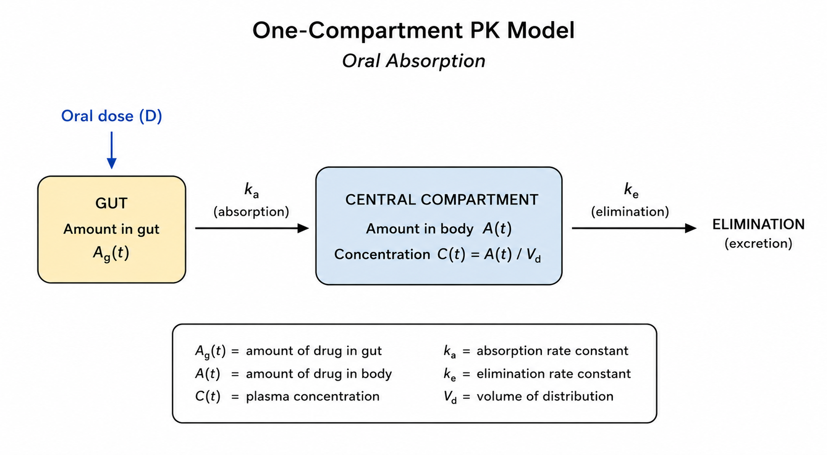
Observed ConcentrationFor an oral one-compartment model, we can simplify this process into compartments.
Note
You may notice that the diagram contains both a gut (absorption) compartment and a central compartment.
The model is still called a one-compartment model because the term refers to the number of body distribution compartments, not the total number of mathematical compartments in the model.
- The gut compartment is a temporary absorption site.
- The central compartment represents the body as a single well-mixed space.
- There is no separate peripheral tissue compartment.
Because the body is represented by only one distribution compartment, this is called a one-compartment oral model.
Interpretation:
- Drug enters through dosing.
- Drug is absorbed into the central compartment.
- Drug leaves through elimination.
- Concentration measurements reflect the amount in the central compartment.
A structural model converts this biological process into equations.
Note
Not all PK models contain an absorption process.
- Oral models typically include an absorption compartment and an absorption rate constant (
ka). - IV bolus models place drug directly into the central compartment.
- Both oral and IV models can be one-, two-, or three-compartment models.
The appropriate structure depends on the route of administration and the observed data.
Observed Profiles vs Structural Prediction
Observed data contain both structure and noise.
Conceptually:
Observed Data = Structural Pattern + Variability + Residual ErrorIn this module, we temporarily focus on only the structural pattern.
Later modules will add:
- interindividual variability
- residual error
- covariates
- estimation
This staged approach helps us understand each model component separately.
Structural Models Can Have Different Structures
The one-compartment oral model shown above is one example of a structural PK model, but it is not the only possibility.
Structural models can differ in both route of administration and the number of compartments used to describe distribution.
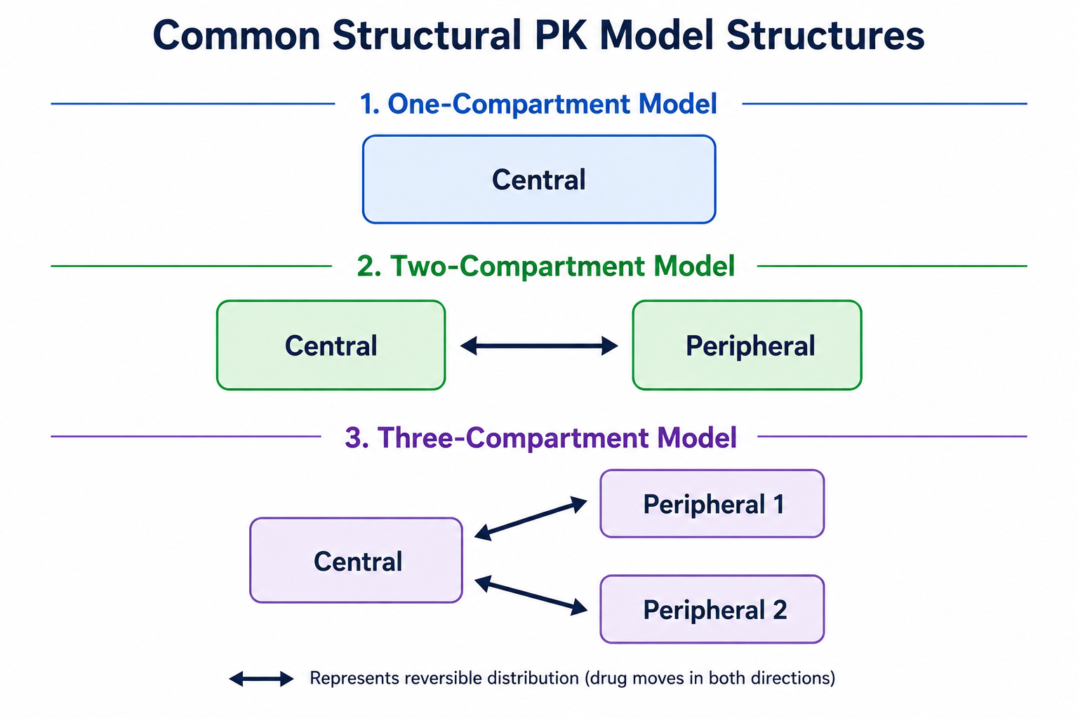
| Model | Typical Use |
|---|---|
| One-compartment | Simple distribution behavior |
| Two-compartment | Distribution into peripheral tissues |
| Three-compartment | More complex distribution behavior |
As model complexity increases, additional compartments may be added to better describe the observed concentration-time profile.
In this course, we will start with simple models and gradually introduce more complex structures when the data justify them.
Worked Example 2: Reading a Concentration-Time Profile
A typical oral PK profile often contains three broad phases.
Rising concentrations
↓
Peak concentration
↓
Declining concentrations
Pharmacometric interpretation:
| Profile Feature | Possible Structural Meaning |
|---|---|
| Rising phase | Absorption dominates |
| Peak | Absorption and elimination balance |
| Declining phase | Elimination dominates |
This interpretation is approximate, but it gives us a starting point for structural thinking.
Structural Models and Parameters
A structural PK model contains parameters with scientific meaning.
Common examples:
| Parameter | Meaning |
|---|---|
ka |
Absorption rate constant |
CL |
Clearance |
V |
Volume of distribution |
k |
Elimination rate constant |
A common relationship is:
\[ k = \frac{CL}{V} \]
This equation connects clearance and volume to the elimination rate.
Worked Example 3: What Changes the Profile Shape?
Structural parameters determine the shape of the concentration-time profile.
To isolate their effects, we change one parameter at a time while keeping the others fixed.
one_comp_oral <- function(time, dose, ka, CL, V) {
  k <- CL / V
  dose * ka / (V * (ka - k)) * (exp(-k * time) - exp(-ka * time))
}

time_grid <- seq(0, 24, length.out = 200)

scenarios <- tribble(
  ~scenario,   ~ka, ~CL, ~V,
  "Reference",  1,   3, 30,
  "Higher CL",  1,   6, 30,
  "Higher V",   1,   3, 60,
  "Higher ka",  2,   3, 30
)

profiles <- scenarios %>%
  rowwise() %>%
  mutate(
    data = list(tibble(
      TIME = time_grid,
      CONC = one_comp_oral(time_grid, dose = 320, ka = ka, CL = CL, V = V)
    ))
  ) %>%
  unnest(data)

ggplot(profiles, aes(TIME, CONC, color = scenario, linetype = scenario)) +
  geom_line(linewidth = 1) +
  scale_linetype_manual(values = c(
    "Reference" = "solid",
    "Higher CL" = "dashed",
    "Higher V" = "dotted",
    "Higher ka" = "dotdash"
  )) +
  labs(
    title = "Effect of Structural Parameters on Profile Shape",
    x = "Time",
    y = "Concentration"
  )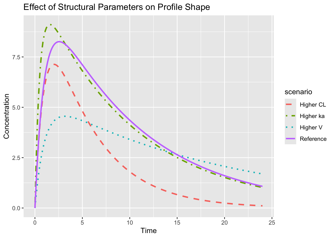
Interpretation:
Higher
CL→ faster elimination
→ lower concentrations over timeHigher
V→ lower initial concentrations
→ slower declineHigher
ka→ earlier peak concentration
These are structural interpretations.
In a population model, individuals may differ in these parameters.
Why Structural Models Come First
A population model contains multiple layers.
Structural Model
↓
Random Effects
↓
Residual Error
↓
Covariates
If the structural model is wrong, adding more variability may hide the problem but not solve it.
For example:
- a one-compartment model may miss a distribution phase
- an absorption model may miss delayed absorption
- a linear elimination model may fail for nonlinear kinetics
This is why structural model selection matters.
Structural Model vs Population Model
A structural model asks:
What curve should the system follow?
A population model asks:
What is the typical curve, and how do individuals vary around it?
So the structural model is not the whole population model.
It is the biological core that the rest of the model builds on.
Connection to nlmixr2
In nlmixr2, the structural model appears inside the model() block.
For example, a future model may include:
model({
  ka <- exp(tka + eta.ka)
  cl <- exp(tcl + eta.cl)
  v  <- exp(tv  + eta.v)

  linCmt() ~ prop(prop.err)
})
For now, do not worry about syntax.
The important idea is that the model block defines how parameters generate predictions.
Strategies
- Start from the observed profile shape.
- Ask what biological processes are visible.
- Keep the first structural model simple.
- Add complexity only when justified.
- Separate structural questions from variability questions.
Common Mistakes
- Jumping directly to estimation.
- Adding random effects to compensate for a poor structure.
- Interpreting parameters without checking the profile.
- Treating a structural model as purely mathematical rather than biological.
Practice Problems
- What does a structural PK model describe?
- Name three biological processes represented in PK structural models.
- Explain what may happen to a concentration profile if clearance increases.
- Explain why structural models should be considered before variability models.
TipStep-by-Step Solutions
Problem 1: What does a structural PK model describe?
A structural PK model describes the expected concentration-time pattern after dosing.
It represents the biological processes that shape the profile, such as absorption, distribution, and elimination.
At this stage, the structural model does not explain all subject-to-subject variability or measurement noise.
Problem 2: Name three biological processes represented in PK structural models.
Common examples include:
- absorption
- distribution
- elimination
For oral PK models, absorption is especially important because drug must enter the systemic circulation before it can be measured as concentration.
Problem 3: What may happen if clearance increases?
Higher clearance usually means drug is removed more efficiently.
If volume remains fixed, increasing CL increases the elimination rate constant:
\[ k = \frac{CL}{V} \]
This leads to faster decline and lower concentrations over time.
Problem 4: Why consider structural models before variability models?
If the structural model is wrong, adding variability can hide the problem rather than solve it.
For example, a poor structural model may show large residual error or unusual individual predictions.
It is better to first ask whether the expected profile shape makes scientific sense.
Summary
- Structural PK models describe expected concentration-time behavior.
- Parameters such as
ka,CL, andVshape the profile. - Structural models come before random effects and residual error.
- Good structural thinking prepares us for population model fitting.
TipQuick Tips
- Start with the profile shape.
- Ask what biology the curve suggests.
- Keep early structural models simple.
- Variability comes later.