library(tidyverse)
library(nlmixr2data)

data("theo_sd", package = "nlmixr2data")

obs <-
theo_sd %>%
filter(EVID == 0)From Structural Model to Population Modeling
Connect structural PK models to the population modeling workflow and introduce structural implementation in nlmixr2.
Tip
Big picture: Structural models describe expected concentration-time behavior. Population models extend this by estimating parameters and quantifying variability.
Learning Objectives
By the end of this lesson, you will be able to:
- Place structural models inside the population modeling workflow.
- Distinguish simulation from estimation.
- Explain how structural models become
nlmixr2models. - Recognize the role of fixed effects and variability.
- Prepare for the first estimated population PK model.
Key Ideas
- Structural models generate expected profiles.
- Population models estimate parameters.
nlmixr2expresses structural assumptions in code.- Estimation adds information from observed data.
Setup
What We Built in This Module
This module started with:
Dose
↓
Structural Assumptions
↓
Parameters
↓
Predicted Concentration
Examples:
- one-compartment oral PK
- parameter interpretation
- simulation
- profile comparison
Now we connect these ideas to population modeling.
Worked Example 1: Simulation vs Estimation
Simulation asks:
What profile would these parameters produce?
Estimation asks:
Which parameters best explain these observations?
Conceptually:
Simulation

Parameters
↓
Prediction
versus
Estimation

Observed Data
↓
Estimate Parameters
↓
Prediction
Worked Example 2: From Structural to Population Thinking
Structural model:
One ProfilePopulation model:
Typical Profile + Variability + Residual ErrorPopulation models estimate:
- fixed effects
- variability
- unexplained error
Worked Example 3: Structural Prediction and Data
Define a structural simulation.
one_comp_oral <- function(time, dose, ka, CL, V){

  k <- CL / V

  dose * ka / (V * (ka - k)) * (exp(-k * time) - exp(-ka * time))

}
Generate prediction.
time_grid <- seq(0,24,length.out=200)

pred <- tibble(
  TIME=time_grid,
  PRED=one_comp_oral(time_grid, 320, 1, 3, 30)
)
Compare with observations.
ggplot() +

geom_point(data=obs, aes(TIME,DV), alpha=.25) +
  geom_line(data=pred, aes(TIME,PRED), linewidth=1.2) +
  labs(
    title="Observed Data and Structural Prediction",
    x="Time",
    y="Concentration"
    )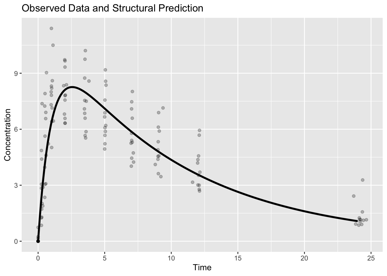
Interpretation:
Observed data vary.
Structural prediction represents expected behavior.
Worked Example 4: Writing the Same Model in nlmixr2
Until now we represented models as R functions.
nlmixr2 expresses the same structural assumptions differently.
library(nlmixr2)

one_comp_model <- function(){

  ini({
    tka <- log(1)
    tcl <- log(3)
    tv  <- log(30)
  })

  model({
    ka <- exp(tka)
    cl <- exp(tcl)
    v  <- exp(tv)

    linCmt() ~ add(0.1)
  })

}
Interpretation:
ini()→ initial valuesmodel()→ model definitionlinCmt()→ analytic compartment solutionadd()→ residual error
Do not focus on the exact syntax yet.
This last line simply tells nlmixr2 how concentrations are generated and how residual error will be represented.
The individual pieces will be introduced in later modules.
Notice:
The concepts did not change.
Only the implementation changed.
Worked Example 5: What Happens Next?
Next module:
Structural Model
↓
Observed Data
↓
FOCEi Estimation
↓
Parameter Estimates
↓
Predictions
↓
Diagnostics
This is where population modeling begins.
Structural vs Population Models
| Structural | Population |
|---|---|
| Known parameters | Estimated parameters |
| One profile | Many profiles |
| Simulation | Estimation |
| No variability | Includes variability |
Strategies
- Build structure first.
- Estimate second.
- Add complexity gradually.
Common Mistakes
- Treating
nlmixr2as magic. - Forgetting assumptions.
- Overfitting early.
Practice Problems
- Explain simulation vs estimation.
- Explain what
ini()does. - Explain what
model()does. - Explain what
linCmt()represents. - Describe what will happen in the next module.
TipStep-by-Step Solutions
Problem 1: Explain simulation vs estimation.
Simulation starts with known or assumed parameter values and generates predicted outcomes.
Estimation starts with observed data and searches for parameter values that explain those data.
So simulation asks, “What would happen if these parameters were true?”
Estimation asks, “What parameters are supported by the data?”
Problem 2: Explain what ini() does.
In an nlmixr2 model, ini() defines initial parameter values.
These include starting values for fixed effects, variability terms, and residual error terms.
Later, estimation will update some of these values based on the data.
Problem 3: Explain what model() does.
The model() block defines how parameters generate predictions.
This is where the structural model, individual parameters, and residual error model are written.
Conceptually, this block connects parameters to predicted concentrations.
Problem 4: Explain what linCmt() represents.
linCmt() represents a built-in analytic compartment model solution.
It allows nlmixr2 to generate concentration predictions without manually writing the full closed-form equation.
The details of linCmt() will be introduced later.
Problem 5: Describe what will happen in the next module.
The next module will take the structural model and fit it to observed data.
Instead of choosing parameters manually, we will let nlmixr2 estimate parameters from theo_sd.
This begins the transition from structural simulation to population model estimation.
Summary
- Structural models generate expected profiles.
- Population models estimate parameters.
nlmixr2expresses structural assumptions in code.- The next module begins actual estimation.
TipQuick Tips
- Simulate first.
- Estimate later.
- Structure before variability.
- Software follows concepts.