library(tidyverse)Delayed Response and ODE Intuition
Introduce delayed pharmacodynamic responses and develop intuition for turnover and ordinary differential equations.
Tip
Big picture: Not all responses occur immediately. Delayed responses motivate dynamic models and introduce ODE thinking.
Learning Objectives
By the end of this lesson, you will be able to:
- explain delayed pharmacodynamic response
- distinguish direct and delayed effects
- interpret turnover concepts
- understand the meaning of an ODE
- explain the roles of production and loss
Key Ideas
- concentration does not always equal response
- response may accumulate gradually
- delayed response introduces state change
- ODEs describe rates of change
Setup
Why Direct Models Are Not Always Enough
Previously we assumed:
Concentration → ResponseBut many biological systems respond gradually.
Examples:
- clotting factors
- biomarkers
- cell populations
Instead:
Concentration

↓

Biological Change

↓

Response
This introduces delay.
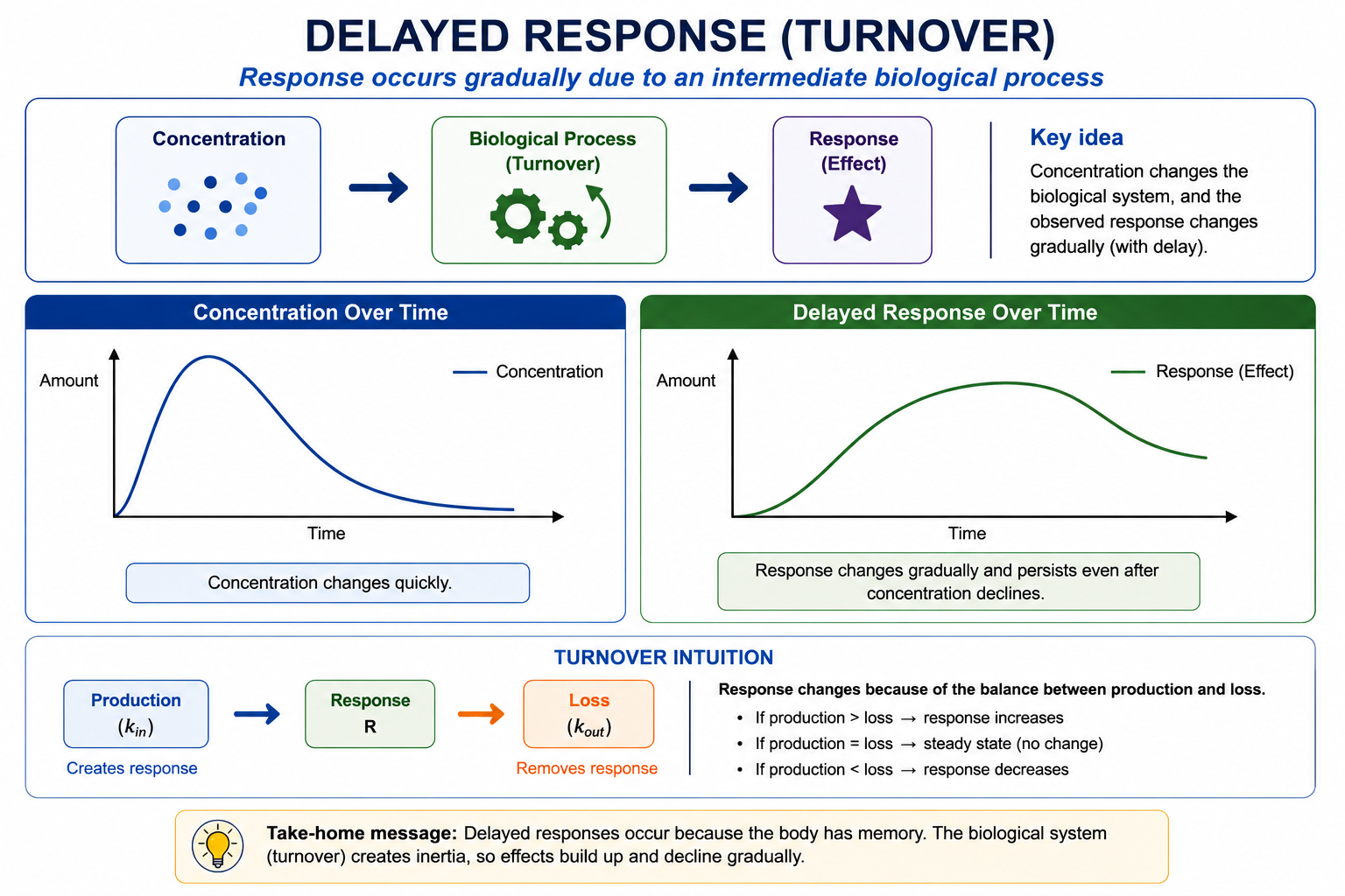
Worked Example 1: Immediate versus Delayed Response
Compare two systems.
Direct effect:
Concentration → EffectDelayed effect:
Concentration

↓

Biological Process

↓

Effect
Question:
Why might effect continue after concentration changes?Answer:
The biological system may have memory.
Worked Example 2: Turnover Intuition
Many responses behave like:
Production

↓

Response

↓

Loss
Examples:
- biomarker synthesis
- protein degradation
- clotting factor turnover
Interpretation:
Response changes because:
Input ≠ OutputWhen:
Production = Lossthe system stays stable.
Worked Example 3: Introducing ODEs
To describe change through time, we introduce an ordinary differential equation (ODE).
The simplest turnover model:
\[ \frac{dR}{dt} = k_{in} - k_{out}R \]
Interpretation:
| Component | Meaning |
|---|---|
| \(R\) | response |
| \(k_{in}\) | production rate |
| \(k_{out}\) | loss rate |
Read this as:
Rate of Change = Production − LossQuestion:
If production exceeds loss,
what happens?
Response increases.
Worked Example 4: Simulate Turnover Behavior
Simulate a simple turnover process.
time <- seq(0, 30, by = 0.1)

kin <- 20
kout <- 0.2

resp <- numeric(length(time))
resp[1] <- 0

dt <- diff(time)[1]

for(i in 2:length(time)) {

  dRdt <-
    kin -
    kout * resp[i - 1]

  resp[i] <-
    resp[i - 1] +
    dRdt * dt
}

turnover_tbl <-
  tibble(
    TIME = time,
    RESPONSE = resp
  )

ggplot(
  turnover_tbl,
  aes(
    TIME,
    RESPONSE
  )
) +
geom_line() +
labs(
  title = "Turnover Response",
  x = "Time",
  y = "Response"
)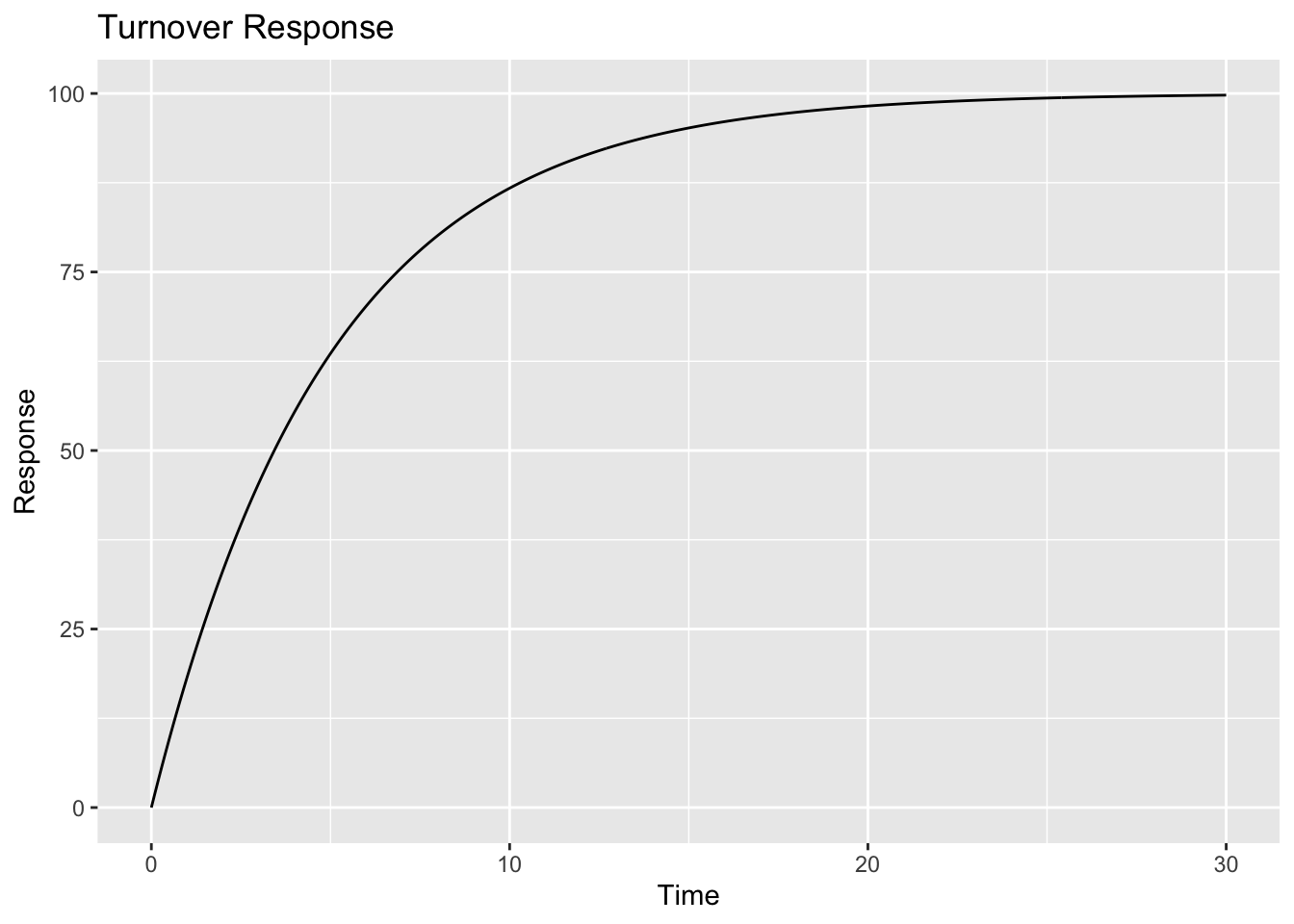
Interpretation:
Response changes gradually.
This pattern is consistent with a turnover process in which response accumulates over time and approaches a steady state.
For now, we focus on the behavior of the system.
Later in the curriculum, we will revisit these ideas when introducing ordinary differential equation (ODE) models and simulation-based approaches.
Worked Example 5: Drug Effect on Turnover
Drugs may influence:
Production → Stimulation or Inhibitionor:
Loss → Stimulation or Inhibition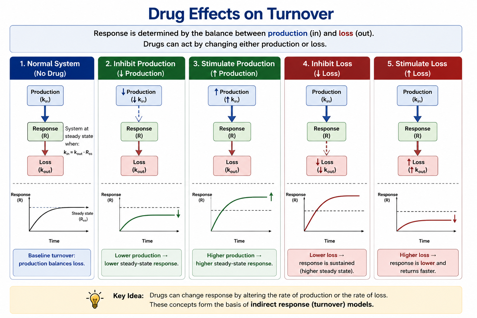
Examples:
| Mechanism | Example |
|---|---|
| inhibit production | lower response |
| stimulate production | higher response |
| inhibit loss | sustained response |
| stimulate loss | faster decline |
This becomes the foundation of indirect response models.
Connecting to PK/PD
Direct models assumed:
Exposure → Immediate ResponseDelayed models assume:
Exposure

↓

Dynamic System

↓

Observed Response
Next lesson combines:
- PK
- PD
- multiple endpoints
using a full PK/PD example.
Strategies
- think about biology
- think about accumulation
- focus on interpretation
Common Mistakes
- treating ODEs as abstract math
- expecting instantaneous response
- ignoring turnover
Practice Problems
What creates delayed response?
What does:
\[ \frac{dR}{dt} = 0 \]
mean?
What happens if production exceeds loss?
Why can direct models fail?
Give one biological example of turnover.
TipStep-by-Step Solutions
Problem 1
Response depends on intermediate biology.
Problem 2
System equilibrium.
Problem 3
Response increases.
Problem 4
They cannot represent delay.
Problem 5
Examples:
- clotting factors
- biomarkers
Summary
- delayed response introduces dynamics
- ODEs describe change
- turnover explains delay
- production and loss determine behavior
TipQuick Tips
- Delay ≠ variability
- ODE = rate of change
- Turnover matters