library(tidyverse)
library(nlmixr2)
library(rxode2)
library(nlmixr2data)

data("theo_sd", package = "nlmixr2data")Simulation Using Fitted Models
Use fitted population models to simulate typical predictions, population predictions, and alternative scenarios.
Tip
Big picture: Estimation creates a model. Simulation turns that model into a prediction engine.
Learning Objectives
By the end of this lesson, you will be able to:
- simulate from fitted models
- distinguish typical and population predictions
- generate future concentration profiles
- simulate alternative scenarios
- interpret model-based predictions
Key Ideas
- simulation can begin from fitted models
- estimation is not repeated
- fitted fixed effects generate typical predictions
- fitted random effects generate population variability
- simulations extend beyond observed data
Setup
This lesson uses fitted models for simulation.
Why Simulate From a Fitted Model?
Earlier lessons used:
rxSolve(model, event)where model was manually defined.
Now we use:
rxSolve(fit, event)where fit contains estimated information from nlmixr2.
Conceptually:
Manual Model

↓

Manual Parameters

↓

Simulation
becomes:
Observed Data

↓

Estimated Model

↓

Simulation
The fitted model contains:
- fixed effects
- random-effect variability
- residual error
- model structure
Simulation uses these estimates to generate predictions.
Worked Example 1: Fit a Population PK Model
Reuse a simple population PK workflow.
one_comp_oral <- function(){

    ini({

        tka <- log(1)
        tcl <- log(3)
        tv <- log(30)

        eta.ka ~ 0.1
        eta.cl ~ 0.2
        eta.v ~ 0.1

        prop.err <- 0.15

    })

    model({

        ka <- exp(tka + eta.ka)
        cl <- exp(tcl + eta.cl)
        v <- exp(tv + eta.v)

        d/dt(depot) = -ka * depot
        d/dt(center) = ka * depot - cl / v * center

        cp = center / v

        cp ~ prop(prop.err)

    })

}
Fit the model.
fit <-
  nlmixr2(
    one_comp_oral,
    theo_sd,
    est = "focei",
    control = list(print = 0)
  )
Interpretation:
The model has learned parameter values from observed data.
Worked Example 2: Inspect the Fit Object
Inspect the fit.
print(fit)── nlmixr² FOCEi (outer: nlminb) ──
OBJF AIC BIC Log-likelihood Condition#(Cov)
FOCEi -298.686 -42.08623 -21.90662 28.04312 30.32751
Condition#(Cor)
FOCEi 9.146425
── Time (sec $time): ──
setup optimize covariance table other
elapsed 0.001616 0.171012 0.171012 0.018 4.10136
── Population Parameters ($parFixed or $parFixedDf): ──
Est. SE %RSE Back-transformed(95%CI) BSV(CV%) Shrink(SD)%
tka 0.38 0.191 50.3 1.46 (1.01, 2.13) 68.6 1.10%
tcl 1.02 0.0728 7.1 2.79 (2.42, 3.21) 24.4 0.108%
tv 3.47 0.0756 2.18 32.3 (27.8, 37.4) 12.5 16.1%
prop.err 0.16 0.16
Covariance Type ($covMethod): r,s
No correlations in between subject variability (BSV) matrix
Full BSV covariance ($omega) or correlation ($omegaR; diagonals=SDs)
Distribution stats (mean/skewness/kurtosis/p-value) available in $shrink
Information about run found ($runInfo):
• gradient problems with initial estimate and covariance; see $scaleInfo
• last objective function was not at minimum, possible problems in optimization
• ETAs were reset to zero during optimization; (Can control by foceiControl(resetEtaP=.))
• initial ETAs were nudged; (can control by foceiControl(etaNudge=., etaNudge2=))
Censoring ($censInformation): No censoring
Minimization message ($message):
relative convergence (4)
── Fit Data (object is a modified tibble): ──
# A tibble: 132 × 22
ID TIME DV PRED RES WRES IPRED IRES IWRES CPRED CRES
<fct> <dbl> <dbl> <dbl> <dbl> <dbl> <dbl> <dbl> <dbl> <dbl> <dbl>
1 1 0 0.74 0 0.74 0.74 0 0.74 0.74 0 0.74
2 1 0.25 2.84 3.00 -0.160 -0.0966 3.39 -0.546 -1.01 2.98 -0.140
3 1 0.57 6.57 5.45 1.12 0.463 6.11 0.462 0.474 5.43 1.14
# ℹ 129 more rows
# ℹ 11 more variables: CWRES <dbl>, eta.ka <dbl>, eta.cl <dbl>, eta.v <dbl>,
# depot <dbl>, center <dbl>, ka <dbl>, cl <dbl>, v <dbl>, tad <dbl>,
# dosenum <dbl>The fit contains:
- parameter estimates
- random-effect variability
- residual error
- prediction information
Earlier lessons required us to manually define values such as:
ka = 1
CL = 3
V = 30
After estimation, these quantities are stored inside the fitted model object.
Simulation therefore becomes:
Fit Once
↓
Reuse Many Times
which is one of the major advantages of model-based analysis.
Question:
Do we need to estimate again before simulating?No.
We already have the fitted model.
Worked Example 3: Simulate a Typical Prediction
Define a future dosing scenario.
ev <-
  et(amt = 300, ii = 24, addl = 6, cmt = "depot") %>%
  et(seq(0, 168, by = 0.5))
Simulate from the fitted model.
sim_fit <-
  rxSolve(fit, ev) %>%
  as_tibble()
Notice that we did not manually specify:
ka
CL
V
omega
All of this information is obtained automatically from the fitted model object.
Plot.
ggplot(sim_fit, aes(time, cp)) +
    geom_line() +
    labs(
        title = "Typical Prediction From Fitted Model",
        x = "Time",
        y = "Concentration"
        )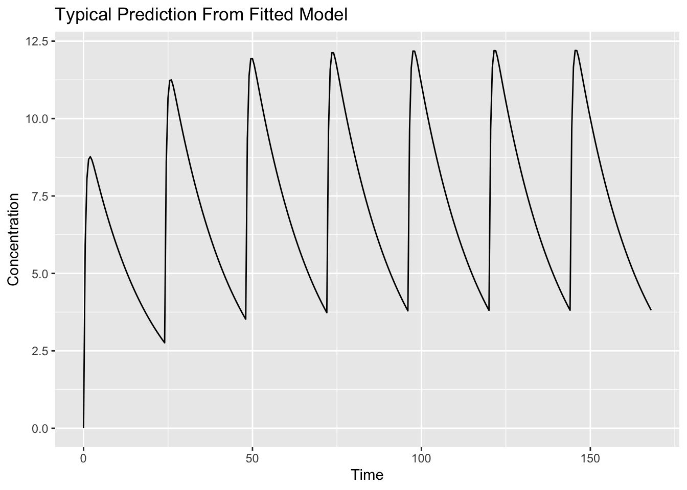
Interpretation:
This profile represents:
Estimated Fixed Effects
↓
Typical Prediction
This simulation uses the fitted model but does not generate a virtual population.
Worked Example 4: Simulate a Population Prediction
Now simulate multiple virtual subjects.
sim_pop <-
  rxSolve(fit, ev, nSub = 100) %>%
  as_tibble()
Unlike earlier population simulations, we do not provide an omega matrix manually.
The estimated variability from the fitted model is already stored inside fit.
When nSub = 100 is requested, rxSolve() automatically uses the estimated variability to generate virtual subjects.
Inspect the simulated subjects.
sim_pop %>%
  count(sim.id)
# A tibble: 100 × 2
sim.id n
<int> <int>
1 1 337
2 2 337
3 3 337
4 4 337
5 5 337
6 6 337
7 7 337
8 8 337
9 9 337
10 10 337
# ℹ 90 more rowsPlot individual simulated profiles.
ggplot(sim_pop, aes(time, cp, group = sim.id)) +
    geom_line(alpha = 0.12) +
    labs(
        title = "Population Simulation From Fitted Model",
        x = "Time",
        y = "Concentration"
        )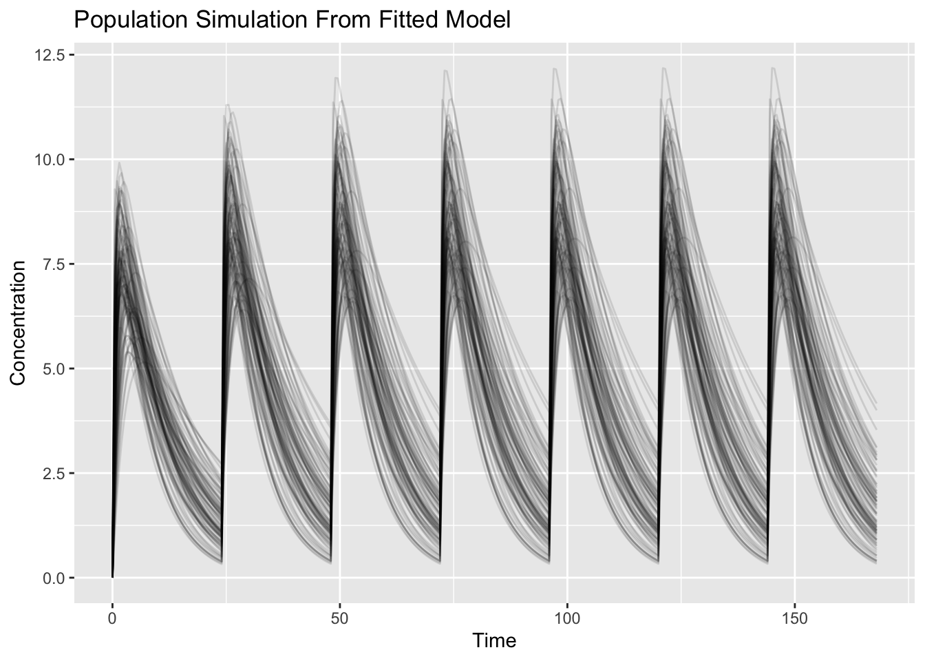
Interpretation:
This simulation uses:
Estimated Fixed Effects
+
Estimated Random Effects
↓
Population Prediction
Each line represents one simulated subject.
Question:
What changed compared with the typical prediction?Variability was added.
Worked Example 5: Compare Population Scenarios
Now compare two dosing scenarios using population simulation.
Define a higher-dose scenario.
ev_high <-
  et(amt = 600, ii = 24, addl = 6, cmt = "depot") %>%
  et(seq(0, 168, by = 0.5))
Simulate both scenarios.
sim_low <-
  rxSolve(fit, ev, nSub = 100) %>%
  as_tibble() %>%
  mutate(SCENARIO = "300 mg")

sim_high <-
  rxSolve(fit, ev_high, nSub = 100) %>%
  as_tibble() %>%
  mutate(SCENARIO = "600 mg")

sim_compare <-
  bind_rows(sim_low, sim_high)
Summarize the population simulations.
sim_summary <-
  sim_compare %>%
  group_by(SCENARIO, time) %>%
  summarise(
    median = median(cp),
    low = quantile(cp, 0.05),
    high = quantile(cp, 0.95),
    .groups = "drop"
  )
Plot scenario summaries.
ggplot(sim_summary, aes(time, median, linetype = SCENARIO)) +
    geom_ribbon(aes(ymin = low, ymax = high, fill = SCENARIO), alpha = 0.15, colour = NA) +
    geom_line() +
    labs(
        title = "Population Scenario Comparison",
        x = "Time",
        y = "Concentration"
        )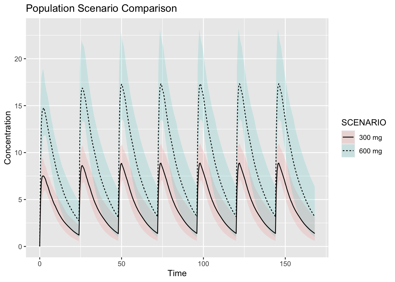
Interpretation:
Ask:
- how much exposure changed?
- did accumulation change?
- did variability overlap?
- are profiles proportional?
Simulation from a fitted model supports scenario comparison using estimated parameters and estimated variability.
Prediction Versus Observation
Simulation predicts.
Observation measures.
Conceptually:
Observed Data

↓

Estimated Model

↓

Predicted Outcomes
Simulation extends beyond observed conditions.
But predictions still depend on:
- model quality
- assumptions
- scenario realism
Connecting to Practice
Simulation from fitted models supports:
- dose selection
- protocol design
- scenario exploration
- model-informed decisions
This is one of the most common pharmacometric workflows.
Looking Ahead
So far:
Estimate

↓

Simulate

↓

Compare
Next we focus on:
Interpret

↓

Communicate
Simulation is useful only if conclusions are meaningful.
Strategies
- fit once
- simulate typical and population predictions
- compare scenarios
- interpret assumptions
Common Mistakes
- assuming simulation is truth
- changing multiple assumptions
- ignoring population variability
Practice Problems
Why simulate from fitted models?
What information does a fit contain?
What is the difference between a typical prediction and a population prediction?
What changes when dose changes?
Why interpret simulations cautiously?
TipStep-by-Step Solutions
Problem 1
To generate predictions using estimated model parameters.
Problem 2
A fit contains:
- fixed effects
- random-effect variability
- residual error
- model structure
Problem 3
A typical prediction uses fixed effects.
A population prediction also includes between-subject variability.
Problem 4
Exposure changes.
Peak concentration, trough concentration, and accumulation may also change.
Problem 5
Predictions depend on model assumptions, model quality, and scenario realism.
Summary
- fitted models support prediction
- typical simulations use fixed effects
- population simulations include variability
- scenarios drive outputs
- interpretation matters
TipQuick Tips
- Fit once
- Simulate typical predictions
- Simulate populations
- Interpret carefully